Processing guide · written 14 November 2026
Seestar & Mak PixInsight Workflow
A complete deep-sky workflow for PixInsight, written for your Seestar S50 and your SVBONY MK127 imaging rig. Each step explains why the process exists as well as which buttons to press, so you can adapt it to any target.
These versions were read from your Mac's PixInsight install, and the RC Astro tools were checked to be running their newest models. Figures captioned Your install are screenshots taken from your own PixInsight on 14 November 2026, set to the values this guide recommends. The other images are from the reference documentation bundled with that install (© Pleiades Astrophoto S.L.), used here for personal study. Numbers marked starting point are typical values to adjust, not fixed rules.
Your two rigs
The single most important number in this guide is image scale: how many arcseconds of sky land on each pixel. (For a feel for how small an arcsecond is, see Appendix C.) It decides whether you drizzle, whether you bin, and how hard you can sharpen. The formula is:
scale (″/px) = 206.265 × pixel size (µm) ÷ focal length (mm)
| Seestar S50 | MK127 + 0.65× reducer + ASI585MC | |
|---|---|---|
| Optics | 50 mm triplet APO, 250 mm, f/5 | 127 mm Maksutov-Cassegrain, ~1500 mm f/11.8 native → ~975 mm f/7.7 with reducer |
| Sensor | Sony IMX462, 1920×1080, 2.9 µm, colour (OSC) | Sony IMX585, 3840×2160, 2.9 µm, colour (OSC), uncooled |
| Image scale | 2.39″/px | ~0.61″/px (1.23″/px after 2×2 binning) |
| Field of view | ~1.28° × 0.72° | ~0.65° × 0.37° |
| Star FWHM | ~3 px measured (7–8″ on your M45 subs; ~2 px on your M31 stack) → adequately sampled. Seeing alone (2–3″) would give ~1–1.3 px, but the Seestar's optics and tracking add blur (see Appendix C) | ~3.5–5 px expected at 2–3″ seeing → oversampled (not yet measured) |
| Mount | Alt-az, so the field rotates during a session | Sky-Watcher GTi (equatorial), guided with UniGuide 32 + ASI120MM Mini in PHD2 |
| What that means | Drizzle 2× only on sharp nights (FWHM under ~2 px in SubframeSelector) with enough subs | Don't drizzle; consider 2×2 software binning |
| Filters | Built-in light-pollution filter (on/off per session) | ZWO Duo-Band 2″ (H-α + O III), or none |
One-time setup
Do these once. Each takes a few minutes and prevents most of the errors people hit later.
- Update PixInsight. Run Resources › Updates › Check for Updates. WBPP 3.2.1 needs core build 1715 or later, so if WBPP complains about the core version, this fixes it.
- Point PixInsight at the Gaia databases. You already have
~/PixInsight-Data/gdr3-1.0.0(astrometry) andgdr3sp-1.0.0(spectra for SPCC). Open Gaia (Process › All Processes), click the wrench (Preferences), and add the.xpsdfiles for DR3 and DR3/SP separately. If SPCC later says "no catalog available", this is the cause. - Finding processes. Every process named here is in Process › All Processes, or type its name into the Process Explorer search. Script menu paths are given in full.
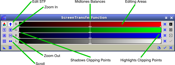
- Turn on the auto-stretch display. Linear images look black. The ScreenTransferFunction (STF) stretches the screen view only without touching the data. Press
Ctrl+A(⌘Aon Mac) on any image. Use the chain icon to link or unlink RGB channels: unlinked hides colour casts, which is useful for judging gradients. - Optional: MARS database for MultiscaleGradientCorrection. MGC is in your install but no
.xmarsfiles were found on your Mac. Without them, use GradientCorrection or GraXpert (both covered below). If you want MGC, download the MARS data from pixinsight.com and add it in MGC's database list.
Part A · Why it works
PixInsight is opinionated about order because each process assumes the data is in a particular state. Understand these five ideas and the workflow stops being a recipe.
Linear vs non-linear data
Straight off the stacker, your image is linear: a pixel's value is proportional to the number of photons it collected. Twice the light gives twice the value. Because faint nebulosity might be 0.1% of the brightness of a star core, almost everything sits in the bottom sliver of the histogram, so the image looks black.
Stretching applies a curve that lifts faint values far more than bright ones. After that the image is non-linear: values no longer track photon counts. You can't go back.
Signal, noise and stacking
Every exposure contains signal (the target) plus random noise (photon shot noise, read noise, thermal noise). Signal adds up in proportion to the number of frames you stack, but random noise only grows with its square root. So:
SNR ∝ √N (N = number of subs, or total integration time)
Four times the integration doubles the SNR. One hour of Seestar 10 s subs is 360 frames; four hours is 1,440. That's also why the Seestar workflow leans on FastIntegration when sub counts reach the thousands.
Stacking does more than average. Pixel rejection compares each pixel across all frames and throws out statistical outliers: satellite trails, planes, cosmic rays and hot pixels that move between frames because of dithering or field rotation.
What calibration frames remove
Darks
Same exposure, gain and temperature as lights, lens capped. They record thermal signal, amp glow and hot pixels, which are then subtracted. Because the ASI585MC is uncooled, its dark current changes with sensor temperature, so darks need to be taken near the same temperature as your lights.
Flats
Evenly lit frames that record vignetting, dust donuts and sensor non-uniformity. These are multiplicative effects, so lights are divided by the normalised master flat. Flats must be shot without changing focus or camera rotation.
Dark flats (or bias)
Darks matched to the flat exposure. They remove the camera's offset from the flats before division; otherwise the flat correction is wrong. For CMOS cameras, dark flats are more reliable than bias frames.
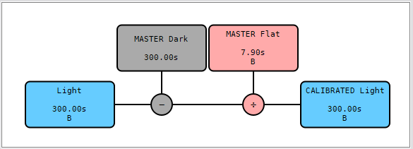
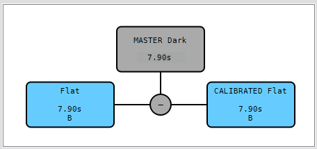
calibrated = (Light − MasterDark) ÷ normalise(MasterFlat − MasterDarkFlat)
Sampling, drizzle and binning
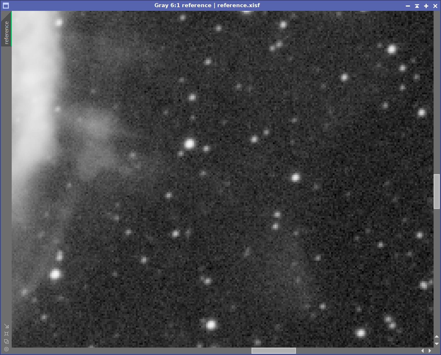
To record a star's shape you need its blur (the FWHM) to span roughly 2–3 pixels. Fewer and stars become blocky squares; more and you're spreading the same light over extra pixels, which adds read noise for no extra detail.
Seestar: few pixels per star on sharp nights
At 2.39″/px, seeing alone would put a star on about one pixel. Your measured subs are softer, about 3 px, which is already well sampled, so drizzle only pays off on nights when SubframeSelector shows stars under about 2 px. On those nights, drizzle integration helps. Each sub lands on the sky slightly shifted (the alt-az mount's tracking drift and field rotation give natural dithering), so drizzle "drops" each input pixel onto a finer output grid. With enough frames, the 2× output recovers real resolution. It needs many subs: plan for at least a few hundred.
MK127: too many pixels per star
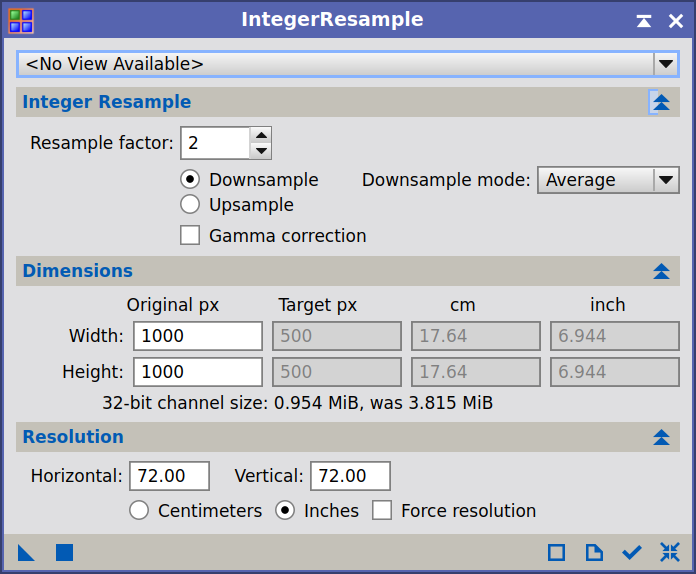
At 0.61″/px, stars are 3.5–5 px wide even in good seeing. Drizzle would only make it worse. Instead you can bin 2×2 in software after stacking (IntegerResample, average). That gives 1.23″/px, halves the file dimensions and doubles the per-pixel SNR with no real loss of detail.
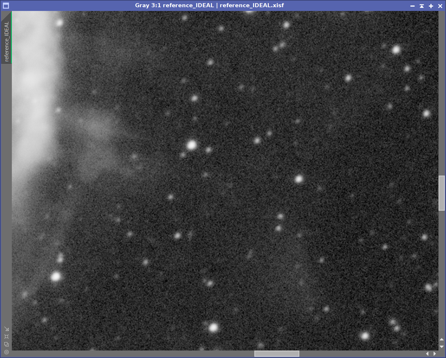
Why the order matters
The diagram shows the order used in Parts B and C. Teal steps run on linear data and red steps after the stretch. The arrows are hard dependencies, not preferences.
Part B · Seestar S50
The Seestar does its own live stacking, but its saved sub-frames contain far more potential. Processing them in PixInsight gets you better rejection, drizzle, proper colour calibration and real deconvolution.
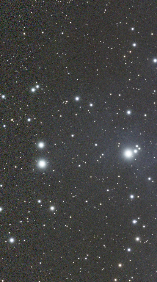
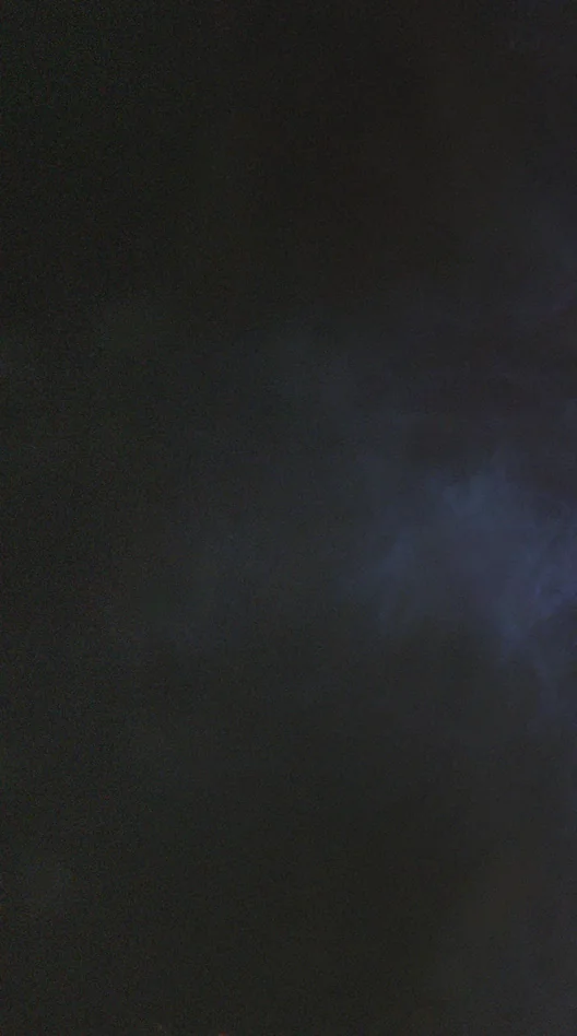
Each step below shows a before/after from your own M45 subs from 31 October 2026, processed with exactly the settings given.
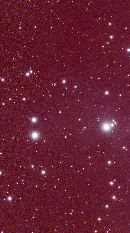
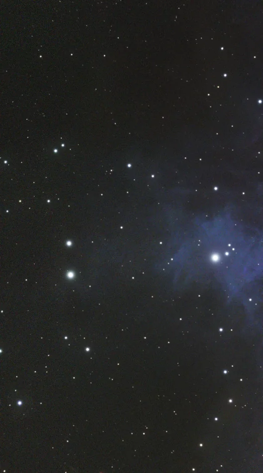
Quick path: start from the Seestar's stacked FITS
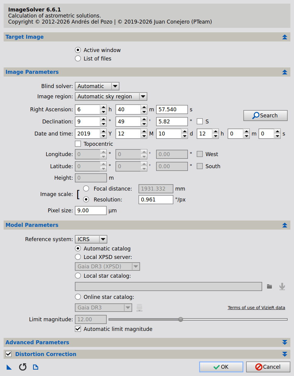
If you only kept the Seestar's own stacked file (Stacked_…fit), you can still use most of this guide. That file is already debayered, rotation-corrected and stacked. Open it, then skip to step 4 (Crop). You'll miss drizzle and pixel rejection, but gradients, SPCC, BlurXTerminator and the rest work. To get SPCC working, plate solve it first with Script › Astrometry › ImageSolver (250 mm, 2.9 µm).
Collect the sub-frames
RAW- In the Seestar app, enable the option to save every sub-frame before you start imaging. Its name varies between app versions; look for "save all frames" or similar in the stacking settings.
- After the session, copy the target's
…_subfolder from the Seestar (it appears as a network or USB drive, underMyWorks) to your Mac. Keep one folder per target and night. - Open one sub and check its FITS header (File › FITS Header, or the Image › FITS Header window). Look for:
BAYERPAT: should readGRBG. WBPP reads it automatically.EXPTIME: usually 10 s (newer firmware allows longer).- Filter and LP-filter state, so you know which SPCC curves to use later.
Inspect and cull bad frames
Blink · SubframeSelectorLINEAROpen Blink, add the subs, and press the auto-STF button so they're visible. Play through them. Delete or move frames with cloud, heavy wind blur, or a dew-fogged lens.
For a measured approach, run SubframeSelector with Subframe scale 2.39 and look at the FWHM, Eccentricity and Stars graphs. A frame with half the normal star count is almost always cloud.
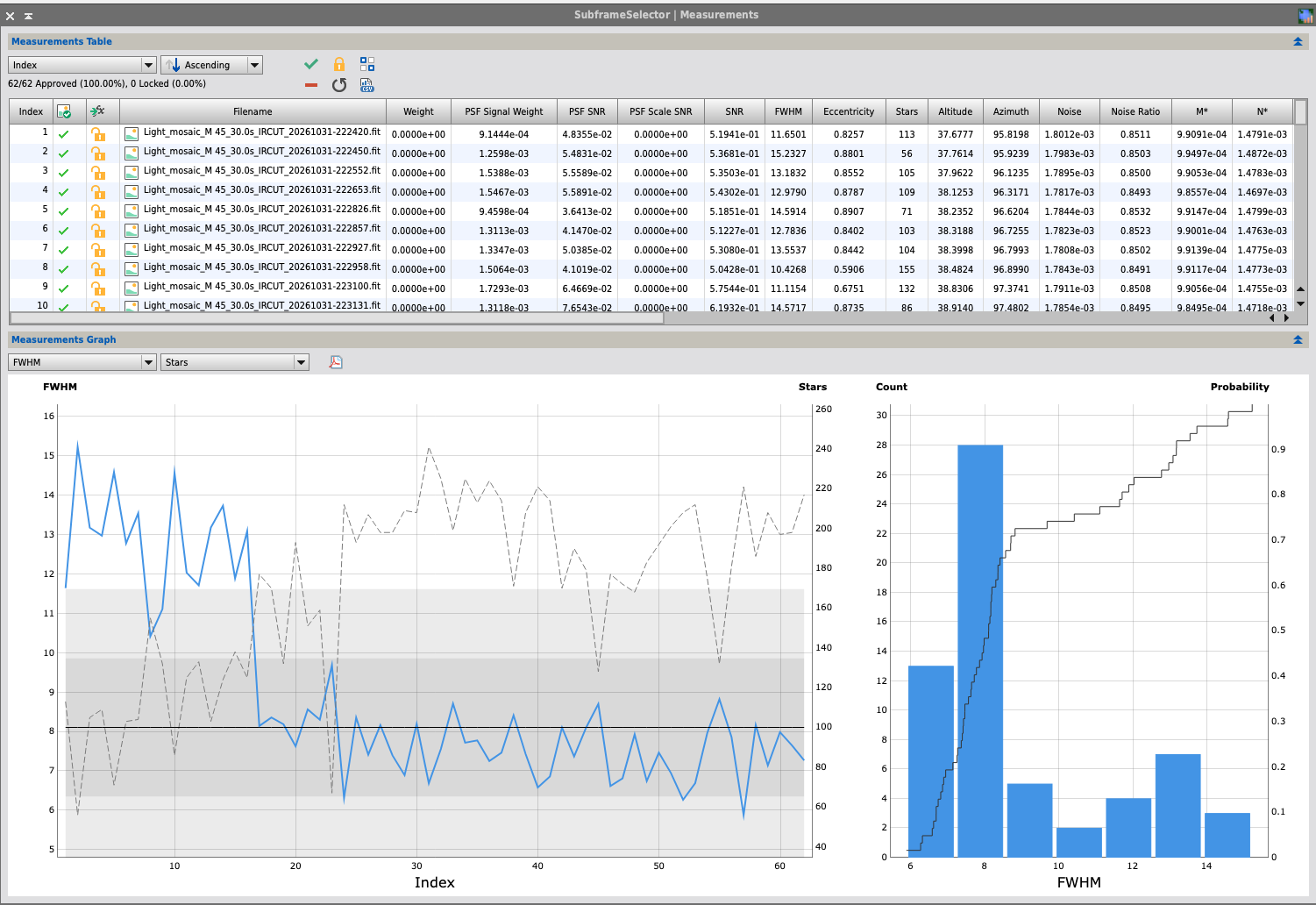
SubframeSelector: every setting explained routine, scale, star detector, expressions
| Setting | What it does | Best practice |
|---|---|---|
| Routine | Measure Subframes measures every frame; Output Subframes writes approved frames with a weight keyword; Star Detection Preview shows what the detector sees on the first frame. | Measure first, inspect the graphs, then either delete bad frames yourself or let WBPP do the weighting. You rarely need Output Subframes when stacking with WBPP. |
| Subframe scale | Image scale in ″/px. Converts FWHM from pixels to arcseconds; only used when Scale unit is arcseconds. | Seestar 2.39 (your solve measured 2.38). MK127 + 0.65×: ~0.61 until you plate solve it. |
| Camera gain | Electrons per data number. Converts noise and SNR figures to electrons; only used when Data unit is electrons. | Leave 1 and Data unit Normalized unless you want absolute noise in electrons. |
| Camera resolution | Bit depth of the subs. | 16-bit for both cameras (12-bit ADC stored as 16-bit). |
| Site local midnight | UTC hour of local midnight, used with DATE-OBS to group frames by night. | Leave 24 (unknown) unless you compare several nights. |
| Structure layers / Noise layers | Wavelet layers for star detection. More structure layers detect bigger stars; noise layers smooth before detection. | Defaults (5 / 0). Raise noise layers to 1–2 only if hot pixels are being counted as stars. |
| Hot pixel filter radius | Median filter applied before detection so hot pixels are not found as stars. | Default 1. Keep it on for the uncooled ASI585MC. |
| Sensitivity / Peak response | Minimum SNR and peakedness for a detection. | Defaults. Lower sensitivity if very few stars are detected on short subs. |
| Maximum distortion | Rejects detections whose shape is far from round (0 round, 1 any shape). | Default 0.6. Raise to ~0.8 if trailed or wind-shaken frames show zero stars and you want to measure them anyway. |
| PSF fit | Function fitted to each star for FWHM and eccentricity (Moffat4 default). | Default. Max PSF fits 8000 is plenty. |
| Approval expression | JavaScript-like test; frames failing it are unapproved, e.g. FWHM < 3.6 && Stars > 120. | Write limits from your own graphs, not generic numbers. For your M45 subs, FWHM < 4 && Stars > 100 (pixel units) rejects exactly the frames culled above. |
| Weighting expression | Formula for a per-frame weight. | Leave blank when stacking with WBPP: WBPP computes its own PSF Signal Weight. |
Source: SubframeSelector parameter tooltips in your PixInsight 1.9.6 install.
Stack with WeightedBatchPreprocessing
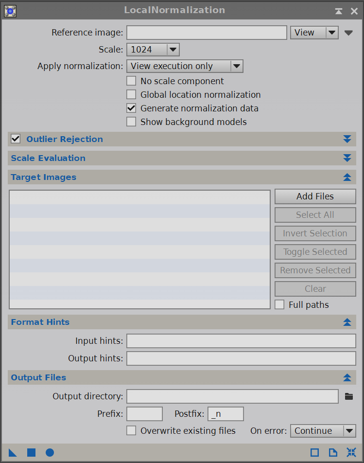
Script › Batch Processing › WeightedBatchPreprocessingLINEARWBPP automates calibration, debayering, measurement, registration, local normalisation and integration. For the Seestar, most of the work is choosing the right options.
| Section | Setting | Why |
|---|---|---|
| Lights | Add Directory → the _sub folder. No bias, darks or flats. | The subs are already dark-subtracted (see step 1). |
| Lights › Debayer | CFA images ✔, Bayer/mosaic pattern Auto, method VNG | Auto reads BAYERPAT=GRBG from the header. VNG preserves edges better than bilinear. |
| Lights › Cosmetic correction | Optional: a CosmeticCorrection template with Auto detect on (hot sigma ~3) | Catches residual hot pixels that dark subtraction missed, before they're smeared by debayering. |
| Image Registration | Defaults. Pixel interpolation Auto, or the new Cardinal Quintic B-Spline option in 3.2.1 | Registration also derotates each frame, which handles the Seestar's field rotation. |
| Local Normalization | Enabled (default) | Evens out the sky brightness changes between frames as the target moves through different parts of your light dome. |
| Image Integration | Rejection Auto | With hundreds of frames, WBPP selects a suitable statistical rejection algorithm. |
| Drizzle configuration | Usually off. On sharp nights: Enable ✔, Scale 2, Drop shrink 0.90, Function Square | Recovers resolution only when the subs are undersampled. Your measured Seestar stars are about 3 px FWHM, which is already well sampled, so leave drizzle off (Scale 1) unless SubframeSelector shows stars under about 2 px and you have ~200+ subs. Otherwise the drizzled image is noisier and patterned with no gain in detail. |
| Autocrop | ✔ | Field rotation leaves ragged, partially covered edges; autocrop trims to fully covered pixels. |
| Astrometric solution | ✔ (focal length 250, pixel size 2.9) | Gives the master a plate solution, which SPCC needs. WBPP 3.2.1 solves against Gaia DR3. |
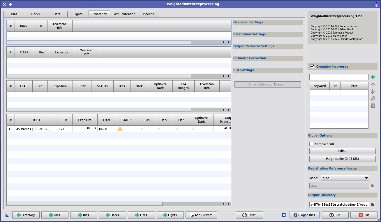
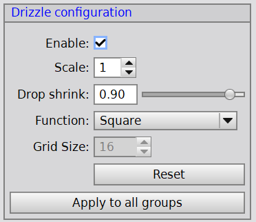

WBPP: the settings that matter rejection, weighting, LN, drizzle, registration
| Setting | What it does | Best practice |
|---|---|---|
| Debayer method | How colour is reconstructed from the Bayer mosaic. | VNG. Bilinear is softer; SuperPixel halves resolution (useful only for the oversampled Mak). |
| Rejection algorithm (Auto) | Removes outlier pixels when integrating. | Leave Auto. WBPP 3.2.1 picks Percentile clipping for ≤ 6 frames, Winsorized sigma for 7–14 and Generalized ESD for 15+. Your 35-frame M45 stack used ESD. |
| Sigma low / high | Clipping thresholds for sigma-type rejection. | Defaults. If satellite trails survive, lower high slightly; if dark pixels or edges look ragged, the low value is too tight. |
| Large-scale rejection | Rejects big bright or dark blobs (planes, clouds) as a unit, not just single pixels. | Turn on high for Seestar sessions near airports or with passing cloud. |
| Subframe weighting | Per-frame weight used during integration. | Default PSF Signal Weight. It rewards sharp, high-signal frames without manual formulas. |
| Minimum weight | Frames below this fraction of the best weight are excluded. | Default. Lower it if WBPPLogAnalysis shows good frames excluded. |
| Local normalization | Matches each frame's background to a reference in a grid, so gradients that change through the night don't confuse rejection. | On. It matters most for alt-az Seestar sessions and multi-night data. |
| Registration reference | Frame all others are aligned to. | auto. For mosaic-mode subs, choose a frame from the panel you want, because frames from other panels may fail to register (10 of yours did). |
| Distortion correction | Spline-based registration that corrects field distortion. | On for mosaics and the reducer-equipped Mak. |
| Drizzle scale / drop shrink / kernel | Output upsampling, size of each dropped pixel, and the shape of the drop. | Seestar with stars under ~2 px FWHM and 200+ subs: scale 2, drop shrink 0.9, Square. Otherwise (including your typical ~3 px Seestar nights) and always on the Mak: drizzle off. |
| Autocrop | Crops the master to the area every frame covers. | On for normal sessions. Off, or use the uncropped master, for mosaic-mode subs. |
| Astrometric solution | Plate solves the master for SPCC/SPFC/MGC. | On, with focal length and pixel size filled in. If it fails, solve manually with ImageSolver (step 7). |
Source: WBPP 3.2.1 scripts and tooltips in your install (rejection rules from BPP-FrameGroup.js).
Pick an output directory and press Run. You'll find the result in master/; with drizzle enabled, use the file whose name includes drizzle.
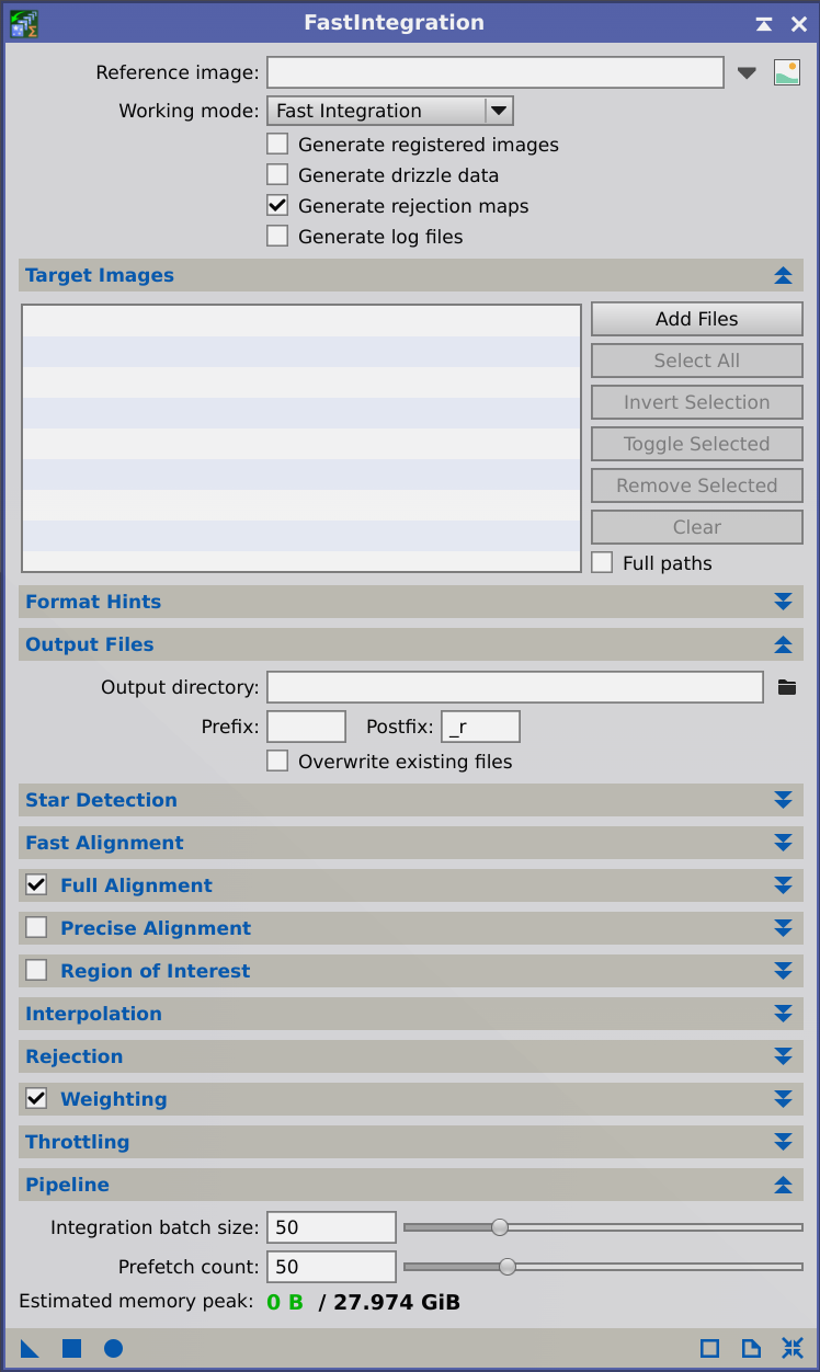
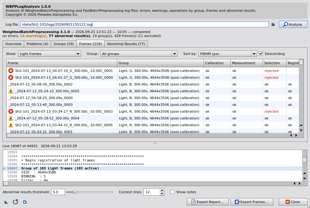
_autocrop in its name, and crop it yourself in step 4. To use all of a mosaic's area, process it as a mosaic instead: see Seestar mosaics.Crop the edges
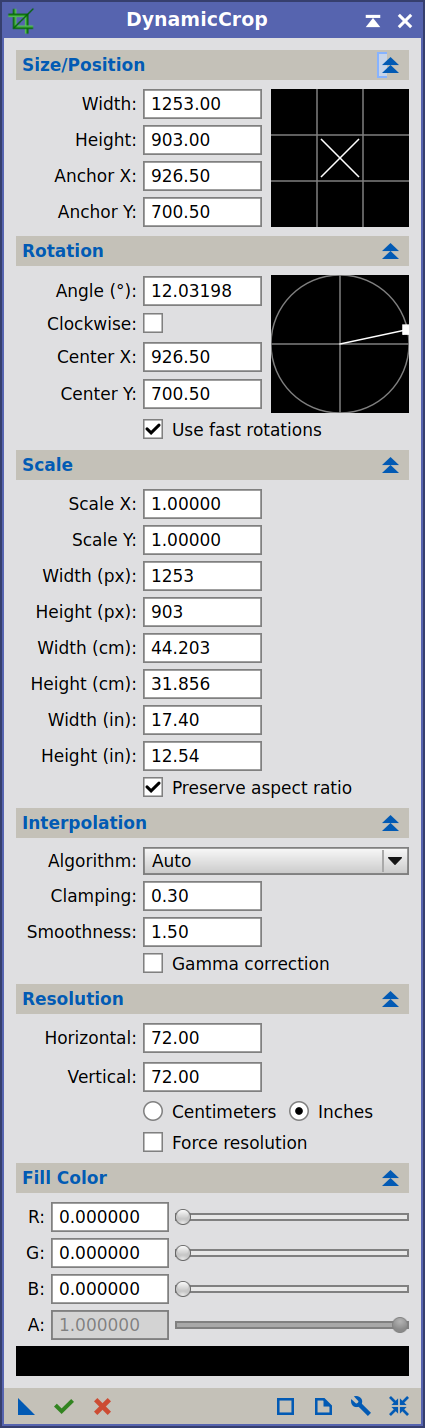
DynamicCropLINEARApply STF auto-stretch and look at the borders. Even after autocrop, there are often a few dark or noisy pixel rows from rotation and drizzle. Open DynamicCrop, drag a rectangle inside the clean area, and apply (green check).
Remove light-pollution gradients
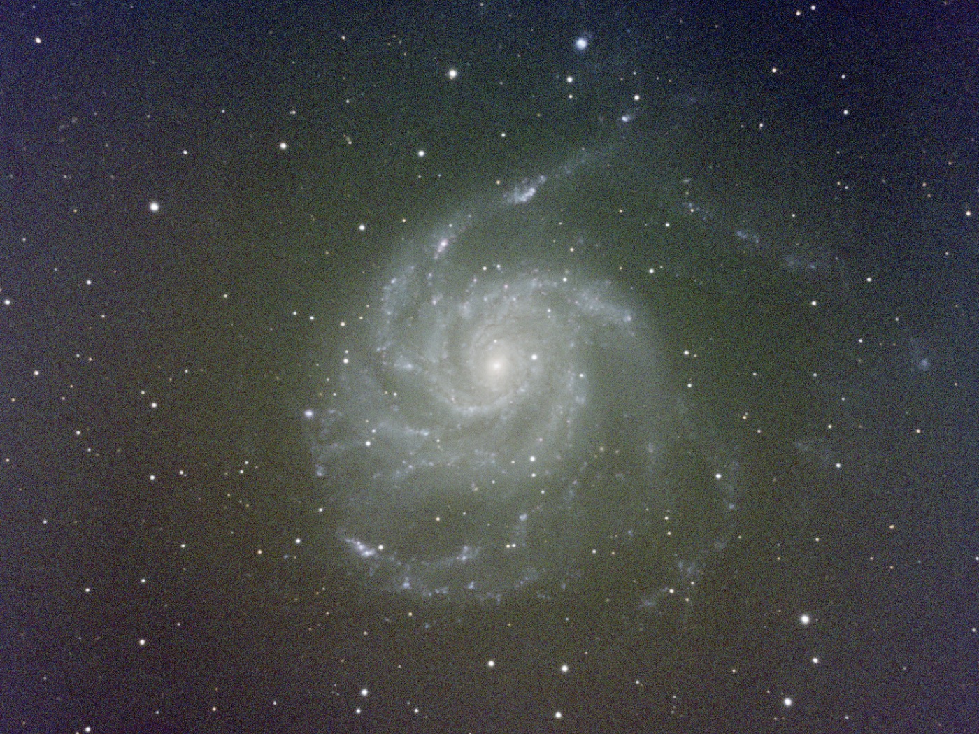
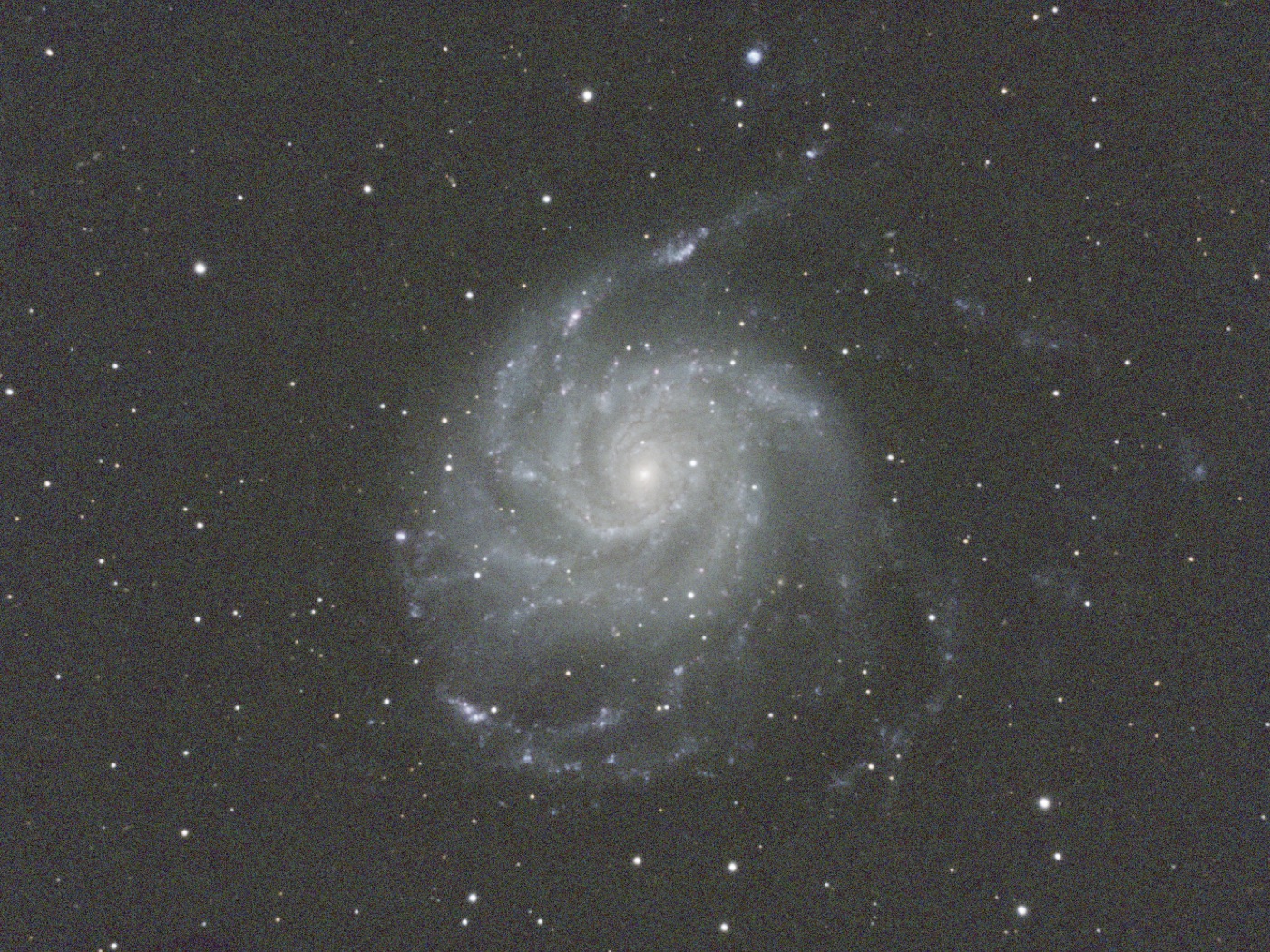
GradientCorrection · GraXpert · MGCLINEARSky glow from towns, the Moon, or low altitude adds an uneven brightness ramp on top of your target. It's additive: it adds to every pixel rather than multiplying, so it has to be subtracted.
Default choice: GradientCorrection
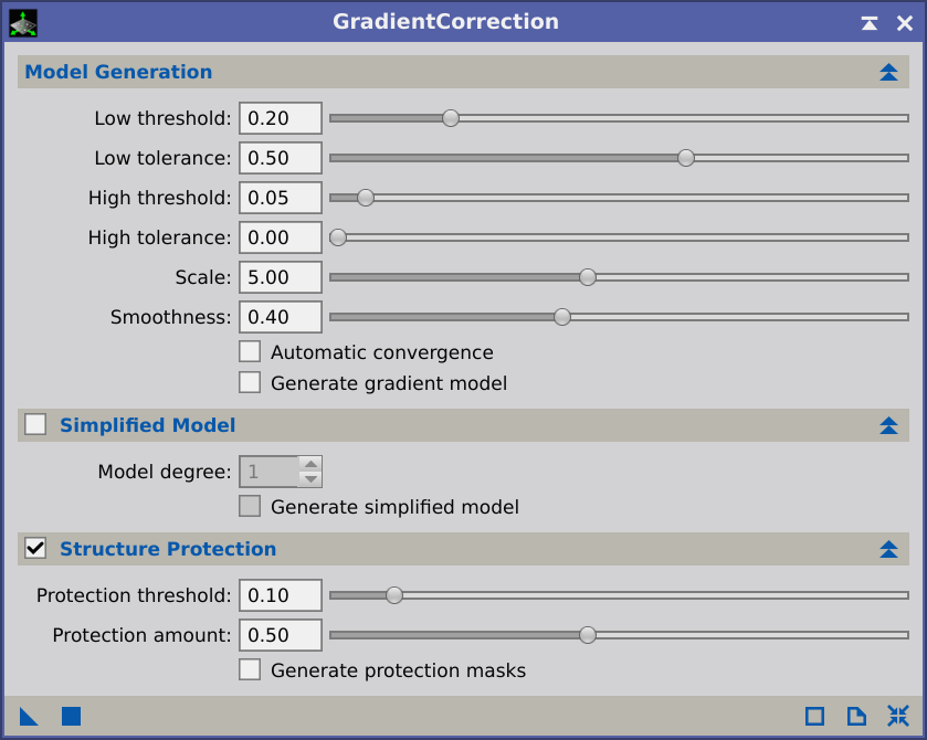
Open GradientCorrection (find it under Process › All Processes, or by typing its name in the Process Explorer search). Start with all defaults and apply. Enable Generate gradient model to see what was removed; it should be a smooth ramp with no trace of your target.
| Parameter | Default | Adjust when |
|---|---|---|
| High threshold | 0.05 | The process's most important control. Raise it if the gradient remains; lower it if the target is being eaten (overcorrection). |
| Low threshold | 0.2 | Rarely needs changing. |
| Low tolerance | 0.5 | Lower it in small steps if dark areas are overcorrected. |
| Structure protection | On (threshold 0.10, amount 0.50) | Keep it on for large bright objects (a big galaxy or M42); it stops the model from absorbing them. See the M31 example. |
GradientCorrection: every setting explained thresholds, scale, protection, tuning order
| Setting | What it does | Best practice |
|---|---|---|
| High threshold | How much relatively bright background structure is allowed into the gradient model. Default 0.05. | The most important control. Raise it if a gradient remains; lower it if the target is being eaten. Change in small steps. |
| High tolerance | How strongly the bright structures selected above contribute. | Default. Raise slightly to recover a mild under-correction. |
| Low threshold | How much dark structure is included in the model. Default 0.2. | Lower it if dark nebulae are being flattened. |
| Low tolerance | How strongly dark structures contribute. Default 0.5 is neutral. | Lower below 0.5 only if dark areas are over-corrected and structure protection doesn't fix it; small steps. |
| Scale | Spatial scale of the multiscale analysis. Default 5.0. | Higher for smooth gradients and big nebulae; lower for sharp, complex light-pollution gradients (at the risk of over-correcting small objects). |
| Smoothness | Smoothness of the model. Default 0.4. | Raise together with Scale to protect faint large nebulosity. |
| Automatic convergence | Repeats the correction until the model stops changing (usually 3–6 iterations). | Off by default; try it on stubborn gradients. |
| Simplified model / degree | Removes a low-degree polynomial gradient first, then models the rest. | Use for very bright, complex gradients. Never with "natural" gradients like the Milky Way along one edge. |
| Structure protection: threshold / amount | Builds a mask to stop bright large objects (galaxies, M42) from being subtracted. | Enable when you see a dark halo around the target. Inspect the protection mask so it covers the object, then raise amount if the outskirts are still over-corrected. |
| Generate gradient model | Outputs the subtracted model as an image. | Always check it: it should be smooth, with no trace of your target. |
Tuning order from the docs: try the defaults; if the gradient remains, turn off protection and try the simplified model at degree 1; then raise High threshold until the background is flat; then re-enable protection and tune threshold and amount. Crop dim or noisy edges first: the algorithm is sensitive to sudden brightness changes at the borders.
Source: GradientCorrection reference documentation in your install.
Alternative: GraXpert
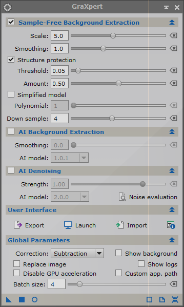
GraXpert is built into your install (Process › All Processes › GraXpert). It uses AI to model the background. It's often excellent on Seestar data with complex, multi-directional gradients (city glow plus the Moon).
Most accurate, if you install MARS: MultiscaleGradientCorrection
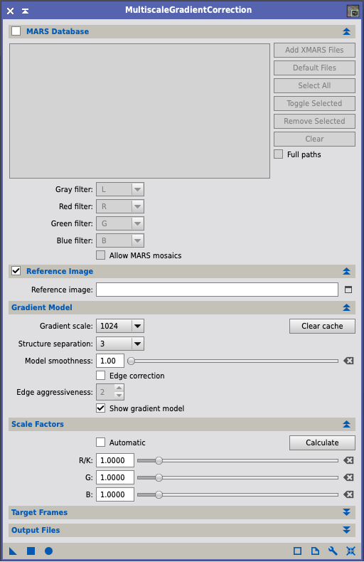
MGC compares your image with professional survey data (the MARS database) to tell real faint nebulosity from sky glow. It needs a plate-solved image and a SpectrophotometricFluxCalibration run first. It's the best option for faint, extended targets, but MARS isn't on your Mac yet (see setup).
.xmars files.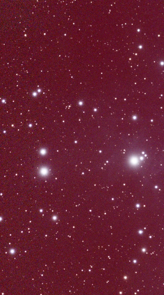
GraXpert and MGC: key settings
| Setting | What it does | Best practice |
|---|---|---|
| GraXpert: Correction | Subtraction or division of the background model. | Subtraction for light pollution. Division only for very strong multiplicative effects such as uncorrected vignetting. |
| GraXpert: AI model | Which neural network models the background. | Reset selects the recommended model. Let downloads finish. |
| GraXpert: Smoothing | Extra blur of the AI background model. | 0.0 in almost all cases. |
| GraXpert: Sample-free scale / threshold | Non-AI mode: size of structures treated as background, and where structure protection starts. | Higher scale protects smaller structures; lower threshold protects fainter structures. |
| MGC: MARS database | Professional survey reference used to separate real signal from sky glow. | Required. Run SPFC first so flux scale factors are correct. |
| MGC: Gradient scale | Largest structure size treated as gradient (default 1024 px). | Lower for complex gradients; keep high to protect large faint nebulae. |
| MGC: Structure separation | How isolated large structures are represented in the model (default 3). | Default; lower to make relative structure intensities more similar. |
| MGC: Scale factors | Per-channel flux scale from SPFC. | Leave at the SPFC values; adjust only if the corrected background is visibly tinted. |
Sources: GraXpert reference documentation and MultiscaleGradientCorrection tooltips in your install.
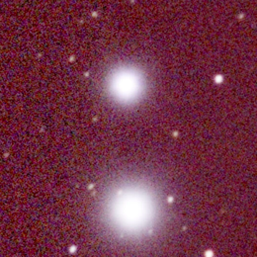
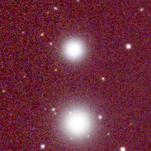
BlurXTerminator: correction pass
BlurXTerminatorLINEARCheck Correct Only and apply. This makes stars round across the field, fixing small amounts of coma, astigmatism, residual chromatic aberration, tracking elongation and 2× drizzle artifacts, without sharpening.
Colour calibration with SPCC
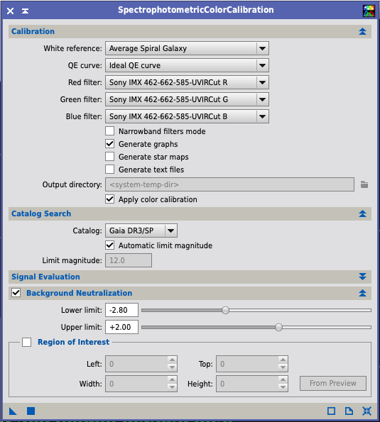
SpectrophotometricColorCalibrationLINEARSPCC finds stars in your image, looks up each one's measured spectrum in Gaia DR3/SP, predicts how bright it should appear through your exact filter and sensor curves, and scales R, G and B until your measurements agree. The result is colour that is physically right rather than a matter of taste.
| Setting | Seestar, LP filter OFF | Seestar, LP filter ON |
|---|---|---|
| White reference | Average Spiral Galaxy | |
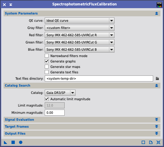
| QE curve | Starting point: Ideal QE curve, the usual choice when the R/G/B curves describe whole camera channels, as these appear to. If the calibration graph looks poor, try Sony IMX585 instead (same sensor family). | |
| Red filter | Sony IMX 462-662-585-UVIRCut R | Seestar-LP-R |
| Green filter | Sony IMX 462-662-585-UVIRCut G | Seestar-LP-G |
| Blue filter | Sony IMX 462-662-585-UVIRCut B | Seestar-LP-B |
| Background neutralization | ✔. Optionally draw a preview on empty sky and set it as the background reference. | |
| Generate graphs | ✔. Points should follow a straight line; a scattered cloud means the fit failed. | |
These curve names are exactly as they appear in your install's filter database.
SPCC: every setting explained references, filters, catalog, photometry
| Setting | What it does | Best practice |
|---|---|---|
| White reference | Spectrum that should come out white. | Average Spiral Galaxy. Hot (blue) references push colour red; cool (red) references push it blue. |
| QE curve | Sensor quantum efficiency, multiplied with the filter curves. | Ideal QE curve when the filter curves already describe the whole camera channel, as the Sony and Seestar curves do. |
| Red / Green / Blue filter | Transmission curve of each colour channel. | Seestar LP off: Sony IMX 462-662-585-UVIRCut. LP on: Seestar-LP. ASI585MC with no filter: the same Sony UVIRCut curves. |
| Narrowband filters mode | Replaces curves with a centre wavelength and bandwidth per channel. | Duo-Band data: H-α 656.3 nm and O III 500.7 nm, bandwidths from ZWO's spec sheet. |
| Catalog / limit magnitude | Gaia DR3/SP spectra source and faintest star used. | Local Gaia DR3/SP with automatic limit magnitude. |
| Background neutralization: lower / upper limit | Background pixels between these limits, in sigma from the median, set the neutral sky. Defaults −2.8 / +2.0. | Defaults. Use a Region of Interest on empty sky if the target fills the frame. |
| Generate graphs | Plots measured against catalog colour ratios for each star. | Always on. A tight straight line is a good fit; a scattered cloud means a bad solve or wrong filters. |
| Saturation threshold | Stars with pixels above this are excluded from photometry. | Default (relative). Keeps clipped Pleiades-type stars out of the fit. |
| PSF growth | Size of the flux-measurement region, in units of the width at one tenth of the peak. Default 1.25. | The tooltip notes that raising it can improve accuracy on undersampled images. Your Seestar stars (~3 px) don't need it; try 1.5 only on unusually sharp nights (under ~2 px) if the graphs look scattered. |
| Minimum SNR / Max stars | Detection limit and cap on measured stars. | Defaults. |
Source: SPCC/SPFC parameter tooltips in your install; Seestar curve names from filters.xspd.
Seestar-LP-R/G/B.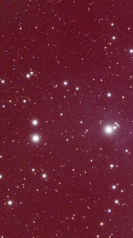
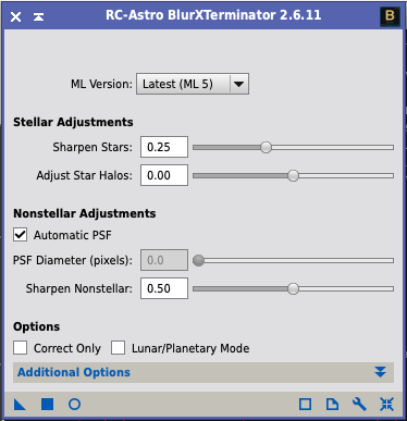
BlurXTerminator: sharpening pass
BlurXTerminatorLINEAR| Control | Seestar starting point | What it does |
|---|---|---|
| Sharpen Stars | 0.20–0.30 | Shrinks star diameter. Too high gives hard dots with dark rings. |
| Adjust Star Halos | 0.00 | Positive softens halos (keeps star colour); negative tightens them. |
| Automatic PSF | ✔ | Measures the blur from stars in each 512×512 tile. Seestar fields have stars everywhere, so this works well. |
| Sharpen Nonstellar | 0.40–0.60 | Sharpens nebulae and galaxies. 1.0 attempts full deconvolution; real detail recovered is limited by SNR. |
| Correct Only | off | Off for this pass. |
BlurXTerminator: every setting explained stellar, nonstellar, options, input rules
| Setting | What it does | Best practice |
|---|---|---|
| Sharpen Stars | Reduces star diameter (FWHM). | 0.20–0.30. If dark rings appear, lower it or raise Adjust Star Halos. High values on long-focal-length data leave flat patches around bright stars. |
| Adjust Star Halos | Brightens (+) or tightens (−) star halos. | 0 for the Seestar; −0.05 to 0 for the Mak's obstruction halos. Raising halos while shrinking stars keeps the colour of stars with clipped cores. |
| Automatic PSF | Measures the blur from stars in each 512 × 512 tile. | On when stars cover the whole field. Off for galaxy cores or star-poor areas, which would otherwise be over-sharpened. |
| PSF Diameter | Manual FWHM (pixels) for nonstellar sharpening. | Set to the measured star FWHM (SubframeSelector or a PSF measurement). Maximum 8 px; data above that is 2× oversampled and should be binned. |
| Sharpen Nonstellar | Fraction of the PSF to remove from nebulae and galaxies; 1.0 tries for a point PSF. | 0.4–0.6. Real gain is limited by SNR. |
| Correct Only | Makes stars round (coma, tilt, astigmatism, CA, guiding, 2× drizzle pairing) without sharpening. | First pass, before SPCC. RC Astro found SPCC fits more consistent after it. |
| Luminance Only | Deconvolves only luminance. | Off. Only for forcing colour retention; disables chromatic corrections. |
| ML Version | Neural-network model. | Latest (ML 5 in your install). |
Input rules from the manual: linear data only (a hard rule with AI4 and later), 32-bit float, no noise reduction before it, and no classical deconvolution before or after it. Remove stars after BXT. For mosaics like your M45 subs, the manual recommends Correct Only on each panel before assembly, then re-solving, then SPCC and sharpening on the assembled mosaic.
Source: BlurXTerminator reference documentation in your install (© RC Astro).
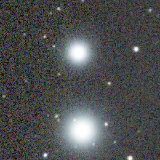
Separate the stars
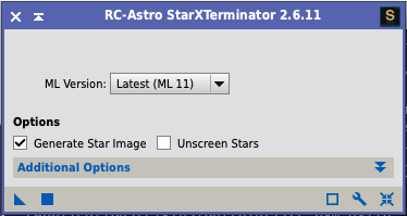
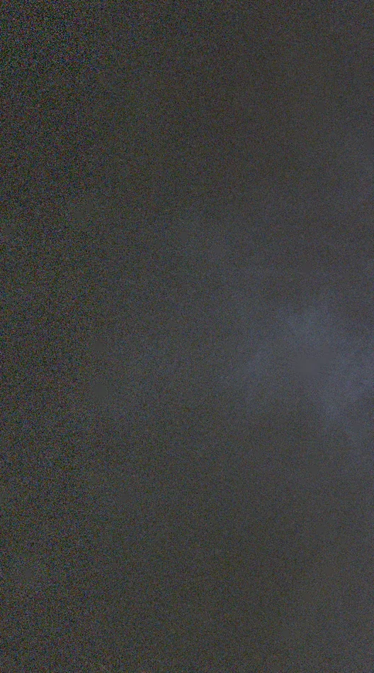
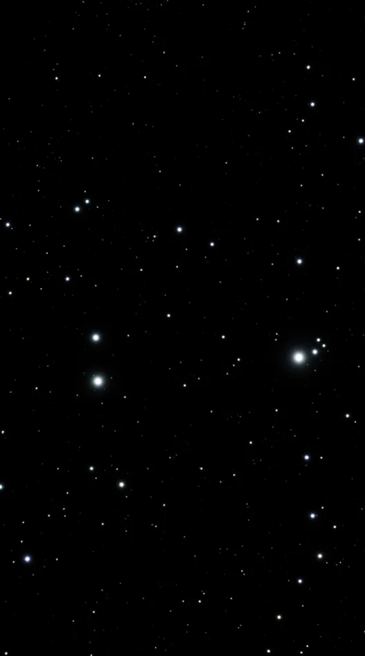
StarXTerminatorLINEARApply StarXTerminator with Generate Star Image ✔ and Unscreen Stars off. You get two images: a starless one and a stars-only one. Both stay linear.
StarXTerminator: every setting explained and how to recombine
| Setting | What it does | Best practice |
|---|---|---|
| Generate Star Image | Creates a stars-only image alongside the starless result. | On whenever you plan to put stars back. |
| Unscreen Stars | Builds the star image so a screen blend reverses the removal exactly. | Stretched (non-linear) images only. Off on linear data, where the star image is original − starless. |
| ML Version | Neural-network model. | Latest (ML 11). |
| Overlap | Overlap between processing tiles (default 0.20). | Default. Raise if you see tile seams. |
Usage notes from RC Astro: run it as early as possible, ideally on linear data after deconvolution, because ArcsinhStretch, GHS, MaskedStretch and HDR processing change star profiles enough that stars may not be recognised. Don't auto-STF the stars image. Stretch the starless and stars images separately, then combine with a screen blend (step 13).
Source: RC Astro StarXTerminator usage notes (rc-astro.com).
Stretch to non-linear
MultiscaleAdaptiveStretch · HistogramTransformation · GHSTHE STRETCHThis is the point of no return. For the theory behind this step, see Appendix A (histograms) and Appendix B (stretching). Save a linear copy (…_linear.xisf) first.
Starless image: MultiscaleAdaptiveStretch (new in 1.9.x)
| Parameter | Default | Guidance from the docs |
|---|---|---|
| Target Background | 0.15 | 0.10–0.20 looks natural. Lower gives a darker sky. |
| Aggressiveness | 0.7 | Black-point clipping. Higher is brighter but noisier. |
| Dynamic range compression | 0.4 | Higher softens bright cores (useful for M42). |
| Contrast Recovery | — | Turn it on. The docs call it "a necessary step in most images", especially with high dynamic range compression. |
| Color Saturation | optional | Includes protection against background chroma noise. |
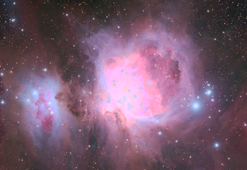
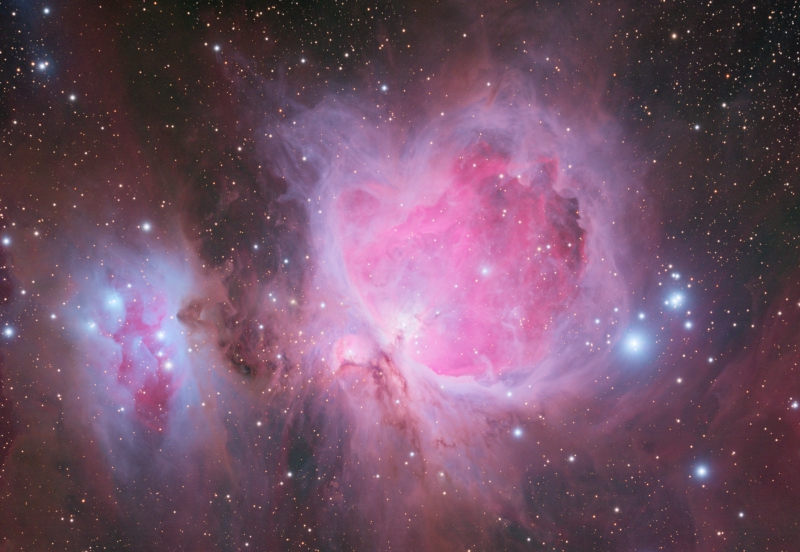
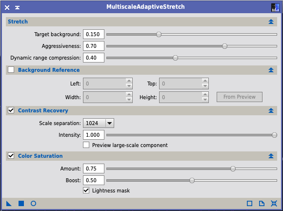
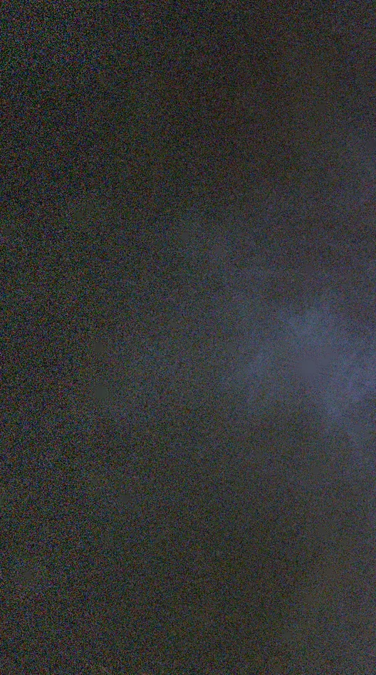
MultiscaleAdaptiveStretch: every setting explained stretch, background ROI, contrast recovery, saturation
| Setting | What it does | Best practice |
|---|---|---|
| Target Background | Background level after the stretch (0–0.5). Default 0.15. | 0.10–0.20 for most targets. Raise to 0.20–0.30 for faint targets or short integrations; 0.25–0.40 when the object fills the frame. Above ~0.25 looks washed out. |
| Aggressiveness | Black-point clipping: how close to the sky peak the clip sits. Default 0.7. | 0.4–0.8 normally. Higher gives more contrast but a noisier background; your M45 needed 0.95. |
| Dynamic range compression | Compresses bright areas to keep star profiles and cores. Default 0.4. | Lower (0–0.4) for gentle targets; raise (0.7+) to protect bright cores. 0 equals a plain MTF stretch. |
| Background Reference | Region used to measure the background. | Use a preview on empty sky when the target fills the frame (M42, Veil). |
| Contrast Recovery | Multiscale recovery of fine contrast lost to compression. | On for nebulae and galaxies. Don't judge it on a small preview: results depend on image size. |
| Scale separation | Boundary between "fine" and "large" structures (8–1024 px). | 128–256 for most images; 512–1024 to also protect large nebulosity. The docs' M45 example raises it to protect bright stars. |
| Intensity | Strength of contrast recovery. Default 1.0. | Reduce if bright cores show artifacts. |
| Color Saturation: Amount / Boost | Saturation curve in HSV; Boost shifts it toward faint colours. | Amount 0.6–0.7 to start. Disable for HDR targets and add colour later with Curves. |
Troubleshooting from the docs: background too grey → raise Aggressiveness or lower Target Background. Too noisy → lower Aggressiveness. Extended objects too dim → raise Target Background.
Source: MultiscaleAdaptiveStretch reference documentation in your install.
Stars image: a gentler stretch
Use ArcsinhStretch (it keeps star colour; see Appendix B) or HistogramTransformation with a moderate midtones move. Stop when the faint stars appear. Over-stretching stars produces big white blobs.
ArcsinhStretch and HistogramTransformation: key settings for the stars image
| Setting | What it does | Best practice |
|---|---|---|
| Arcsinh: Stretch factor | Logarithmic slider 1–1000; noise is amplified by the same factor. | Stars image: 10–50. For more than 1000, run it twice (three runs of 6.7 ≈ one run of 300). |
| Arcsinh: Black point | Coarse and fine sliders; values below are clipped. | In the real-time preview, click Estimate Black Point (clips 2%), then fine-tune. |
| Arcsinh: Protect highlights | Scales the image so no channel clips. | On for stars; the result is a little darker. |
| Arcsinh: Use RGB working space | Luminance weights for the stretch. | Off (equal weights). |
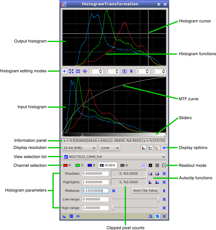
| HT: Shadows / Midtones / Highlights | Black point, MTF balance and white point. | For the stars image, midtones only (your M45 used 0.04) and no clipping. Watch the clipped-pixel count when moving shadows. |
Turn the STF off before using ArcsinhStretch's preview: an active STF distorts what you see.
Source: ArcsinhStretch and HistogramTransformation reference documentation in your install.
Manual alternative: HistogramTransformation from the STF
Apply STF auto-stretch, then drag the STF's triangle icon onto HistogramTransformation's bottom bar, and apply HT to the image. This makes the screen stretch permanent. It's quick but blunt; GeneralizedHyperbolicStretch gives finer control.
Noise reduction
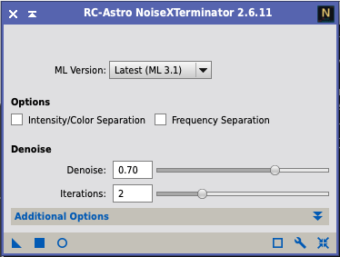
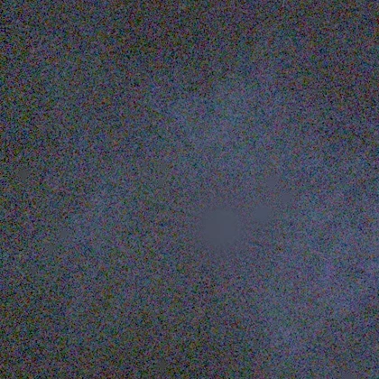
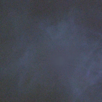
NoiseXTerminatorNON-LINEARApply NoiseXTerminator to the starless image. Starting point: Denoise 0.6–0.8, other options at defaults. Compare the result with the original by zooming to 1:1 on faint areas.
NoiseXTerminator: every setting explained denoise, iterations, separation
| Setting | What it does | Best practice |
|---|---|---|
| Denoise | Fraction of noise removed (0–1). | 0.6–0.85. RC Astro warns that 1.0 can look unnaturally smooth. |
| Iterations | Successive-approximation passes (AI3 only). | Default 2. More can recover detail in very noisy areas but may add artifacts; inspect carefully. |
| Intensity/Color Separation | Separate sliders for brightness noise (Denoise) and colour noise (Denoise Color). | Colour noise is more objectionable: set colour higher than intensity, e.g. 0.75 / 0.95. |
| Frequency Separation | Separate sliders for fine (HF) and blotchy (LF) noise, split at the HF/LF scale. | LF usually lower than HF, especially on dust and faint nebulae. Tune the scale with Denoise LF at 0 in the real-time preview. |
| Both separations | Four sliders: HF intensity, HF colour, LF intensity, LF colour. | RC Astro's starting point: HF intensity 0.80–0.90, HF colour 0.90–1.00, LF intensity 0.50–0.70, LF colour 1.00. |
| Detail | Sharpening during denoising. | AI2 only; no effect on the current model. |
| ML Version | Model. | Latest (ML 3.1). |
From the manual: works equally on linear and stretched data (it stretches internally). Never before deconvolution of any kind. Use the real-time preview: the right amount is subjective.
Source: RC Astro NoiseXTerminator 2 AI3 user manual (rc-astro.com).
Contrast and colour
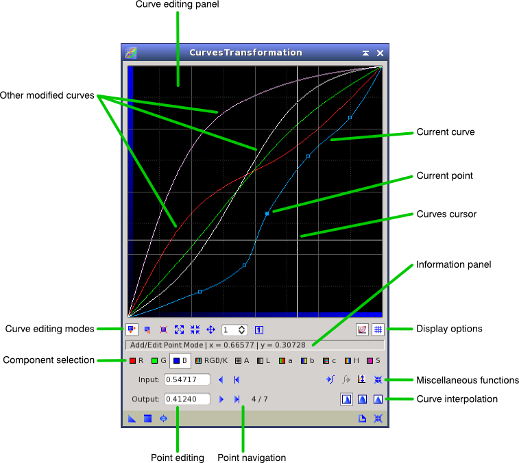
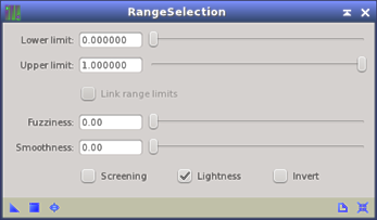
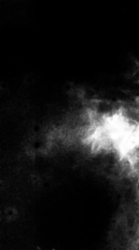
CurvesTransformation · LocalHistogramEqualization · RangeSelectionNON-LINEAR- Make a mask. RangeSelection with Lightness on: lower limit just above the background (read the background median in Statistics and add about one noise σ), fuzziness 0.1–0.2, smoothness 3–5. Apply it with Mask › Select Mask. White areas of the mask are changed; black areas are protected. Mask › Show Mask toggles the red overlay; Mask › Remove Mask when done.
- Curves. Darken the sky with an unmasked RGB/K curve first. Then, with the mask active, a gentle S-curve on
RGB/Kadds contrast and raising theS(saturation) curve boosts colour on the target only. - Local contrast. LocalHistogramEqualization (kernel radius 64–128, amount 0.2–0.4) brings out structure in bright nebulosity.
Curves, LocalHistogramEqualization and RangeSelection: key settings
| Setting | What it does | Best practice |
|---|---|---|
| Curves: RGB/K | Tone curve on all channels. | Gentle S-curve. Pull the lowest point slightly to darken the sky (your M45: 0.20 → 0.13). |
| Curves: S (saturation) | Saturation curve. | Lift the middle a little (0.5 → 0.6–0.65). Use a mask so the background doesn't gain colour noise. |
| LHE: Kernel radius | Neighbourhood size for local histograms. | 32–128. Smaller is stronger but noisier and rings around stars. |
| LHE: Contrast limit | Maximum slope of the local transfer curve. | 1.5–3. Higher approaches plain equalization and boosts noise. |
| LHE: Amount | Blend with the original. | 0.2–0.4 for natural results. Test on previews larger than twice the kernel radius; protect stars with a mask. |
| RangeSelection: Lower / upper limit | Pixel range selected into the mask. | Lower limit just above the background level. |
| RangeSelection: Fuzziness | Softens the limits. | 0.1–0.2 to avoid hard edges. |
| RangeSelection: Smoothness | Gaussian blur of the mask. | 3–5 so the mask follows structures, not noise. |
| RangeSelection: Lightness / Screening / Invert | Build from L*, multiply by the image, or invert. | Lightness on for colour images; invert to protect instead of select. |
Sources: CurvesTransformation, LocalHistogramEqualization and RangeSelection reference documentation in your install.
Put the stars back
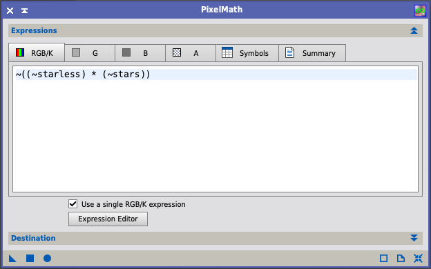
PixelMathNON-LINEAROpen PixelMath, leave Use a single RGB/K expression checked, and enter this expression, replacing the names with your image IDs:
~((~starless) * (~stars))
Under Destination, check Create new image and apply to either image.
1 − (1−a)(1−b). Unlike simple addition, it can never exceed 1.0, so star cores don't clip where they overlap bright nebulosity. It is also the blend RC Astro recommends for putting StarXTerminator stars back after stretching the two images separately.PixelMath: settings for recombining stars
| Setting | What it does | Best practice |
|---|---|---|
| Expression (RGB/K) | Formula evaluated per pixel. ~x means 1 − x. | ~((~starless) * (~stars)): a screen blend. |
| Use a single RGB/K expression | Applies the same formula to all channels. | On for recombination; off for channel mixing (HOO). |
| Rescale result | Stretches the output to fill 0–1. | Off: a screen blend already stays in range, and rescaling changes your tones. |
| Truncate | Clips values outside 0–1. | On (default). |
| Destination: Create new image | Writes to a new window instead of overwriting. | On, with a clear Image ID, so both inputs survive. |
| Symbols | Declares variables for longer expressions. | Not needed here. |
Source: PixelMath parameter tooltips in your install.
Too many stars? Multiply first: ~((~starless) * (~(stars*0.8))).
Save and export
FINAL- Save the master as XISF (32-bit float). That's your archive; everything else is derived from it.
- For sharing: Image › Sample Format › 16-bit (on a duplicate), then save as TIFF for further editing or JPEG (quality 90+) for the web. Make sure the colour profile is sRGB for web use.
- Keep the linear master from step 10. If you learn a better stretch in six months, you start there.
Seestar mosaics
A mosaic covers more sky than one frame by combining frames aimed at different points. The Seestar makes them in two ways: its Mosaic framing mode, which moves between positions during a session, and longer sessions where the alt-az mount and field rotation make the pointing drift. Either way, the subs don't share one field, and a normal WBPP run quietly throws much of the data away.
Signs you have mosaic data
- File names start
Light_mosaic_. - The
RA/DECkeywords differ by more than a few arcminutes between subs. - WBPP reports "registration failed" for some frames, and autocrop leaves a narrow strip.
Your M45 session
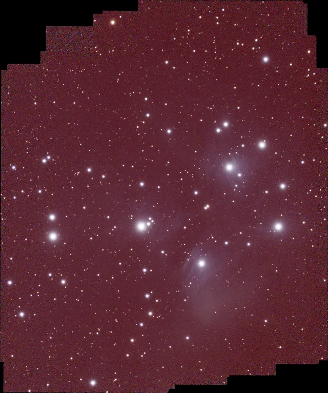
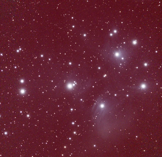
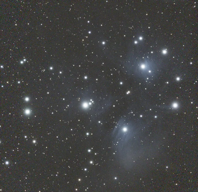
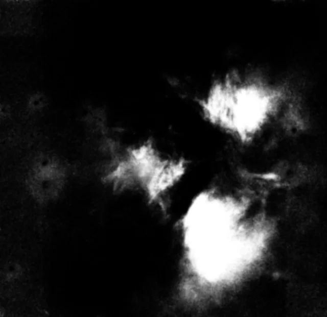
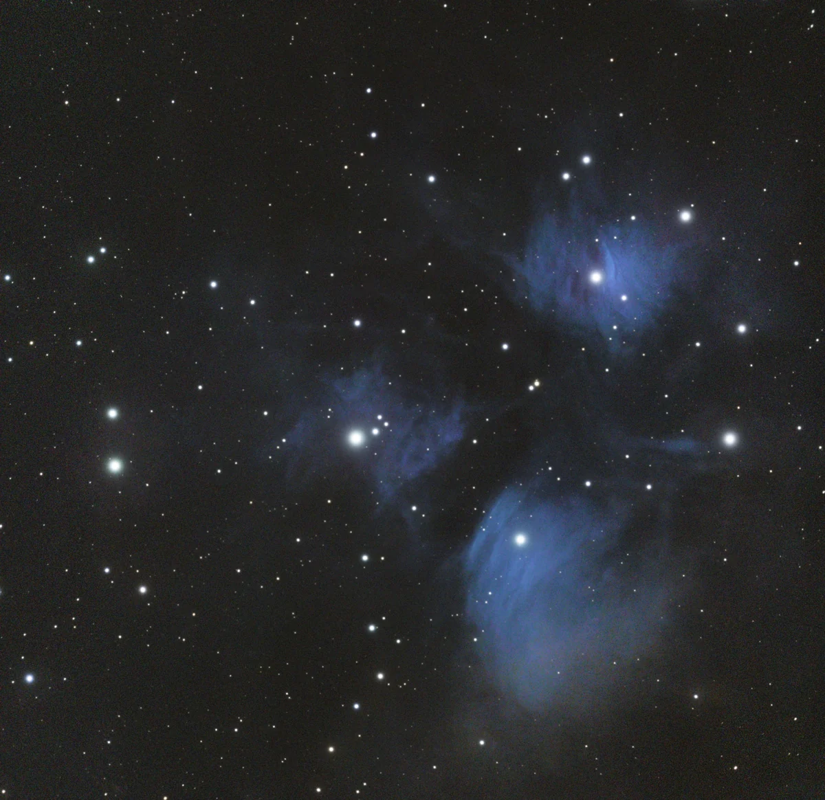
The 45 good subs' pointings spread over about 0.7° × 0.5°. Plain WBPP registered 35 of them and autocrop cut the master to 370 px wide. Processed as a mosaic, all 45 contribute and the field grows from about 0.70° × 1.25° to 1.31° × 1.27°.
For planning a mosaic (coverage, time per panel, targets) see Mosaics with the Seestar in Appendix C.
Route A: put every sub on one canvas (recommended for Seestar subs)
This is what produced the images below. Each sub is plate solved, reprojected onto a common canvas that covers the whole mosaic, and integrated with empty areas ignored.
- Calibrate and debayer only. Run WBPP on the culled subs as in step 3, but with Image Registration and Image Integration off. You only need the
debayeredfolder. - Plate solve every sub. Script › Astrometry › ImageSolver, with the subs added as target files: focal length 250 mm, pixel size 2.9 µm, distortion correction on, local Gaia DR3. All 45 of yours solved.
- Reproject. Script › Astrometry › MosaicByCoordinates: add the solved subs, leave the geometry automatic and press Calculate. Yours gave a 2160 × 2586 px canvas at 2.377″/px. Run it to write one reprojected image per sub.
- Integrate. ImageIntegration on the reprojected images with Clip low range on (range low 0) so the zero-filled areas are ignored, rejection Generalized ESD, normalization Additive with scaling, weights PSF Signal Weight.
- Crop to good coverage. The canvas edges are ragged and covered by only a few subs. Crop to the area most subs cover (step 4), then continue with steps 5–14 on the cropped mosaic. Plate solve the result again before SPCC.
Route B: stack each panel, then merge
Use this when the panels are distinct: planned multi-panel mosaics, panels shot on different nights, or very long sessions where Route A's disk use gets out of hand. It follows the mosaic workflow in BlurXTerminator's manual and the GradientMergeMosaic documentation. I ran it on the same 45 M45 subs, first with autocrop on each panel and then with autocrop off. The recipe below is the version that worked best.
- Group the subs into panels. Read each sub's
RA/DECkeywords and group neighbouring pointings. Keep at least 8 subs per panel, or pixel rejection has too little to work with. The Seestar may revisit a position later in the night, so don't group by time alone. Your session visited about 15 positions with 2–4 subs each; grouping by position gave 4 panels of 8, 14, 8 and 15 subs. - Stack each panel separately in WBPP with normal registration and local normalization, and autocrop off. Autocrop throws away each panel's outer strip, and in a mosaic those strips are the overlaps.
- On each panel master: crop 8 px from the edges, then BXT Correct Only. The corners of neighbouring panels have different aberrations, so they're corrected before the panels meet. Leave gradient correction until after the merge for nebula-rich targets: each panel is small, and the nebula can fill much of it.
- Plate solve each corrected panel with distortion correction and local Gaia.
- MosaicByCoordinates on the panel masters. List the panel you want to set the orientation first.
- GradientMergeMosaic on the reprojected panels: Average, shrink radius 10 (the maximum), feather radius 30, black point 0. Tick Generate Mask to see how the panels overlap.
- Crop to the fully covered rectangle, then GradientCorrection, plate solve, SPCC, BXT sharpening, and steps 9–14.
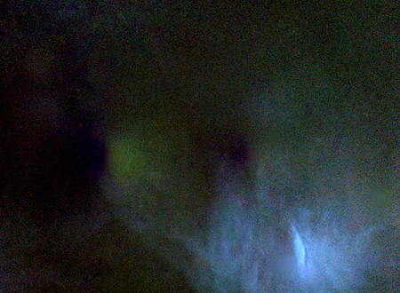
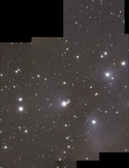

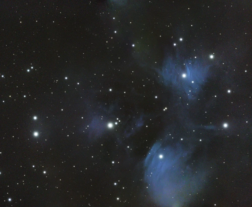
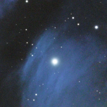
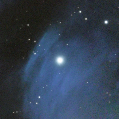
| Route A: one canvas | Route B, autocrop on | Route B, autocrop off | |
|---|---|---|---|
| Subs used | 45 | 45 | 45 |
| Usable field (your M45) | 1990 × 1930 px (1.31° × 1.27°) | 1646 × 1441 px (1.09° × 0.95°) | 1972 × 1620 px (1.30° × 1.07°) |
| Reprojected files | 2.8 GB (one per sub) | 179 MB | 231 MB |
| Seams and artifacts | None: one integration | None visible with defaults | Needs shrink 10 and feather 30 |
| Extra work | Plate solve every sub | Group subs, one WBPP run and plate solve per panel | |
| Best for | Seestar sessions whose pointing drifts; up to a few hundred subs | Distinct panels, multi-night panels, very long sessions | |
MosaicByCoordinates, ImageIntegration and GradientMergeMosaic: key settings for mosaics
| Setting | What it does | Best practice |
|---|---|---|
| MBC: Input images | Solved images to reproject. The first one sets the mosaic's rotation. | Every image needs a solution computed with distortion correction and the local Gaia XPSD databases; online catalogs can't constrain the corners, where tiles overlap. |
| MBC: Projection / Center / Resolution / Rotation / Dimensions | Geometry of the common canvas. Each is automatic unless you tick it. | Leave all automatic and press Calculate to see the canvas size before running. Resolution defaults to the finest input, so never mix in one long-focal-length frame by accident: the canvas grows with the square of the scale ratio. |
| MBC: Pixel interpolation / Clamping | Resampling method and ringing suppression. | Auto (Lanczos-3 for unchanged scale) and clamping 0.3. |
| MBC: Output directory / suffix | Where the reprojected images go (suffix _ra). | A scratch folder with plenty of space: every output has the full canvas size. |
| II: Range rejection, clip low (range low 0) | Excludes pixels at or below the low limit. | Essential. Areas a frame doesn't cover are filled with zeros, and the docs warn that zeros treated as data cause dark seams and depressed backgrounds. |
| II: Rejection | Outlier rejection. | Generalized ESD for 15+ frames per pixel; Winsorized sigma for fewer. |
| II: Normalization | Matches frame levels before combining. | Additive with scaling. |
| II: Weights | Per-frame weighting. | PSF Signal Weight. |
| GMM: Type of combination | Overlay (later images hide earlier ones) or Average (averages overlapping pixels). | Average for panels of similar depth; it also improves SNR in the overlaps. |
| GMM: Shrink radius | Pixels trimmed from each panel's border (0–10). | Default 1 for autocropped panels; 10 for uncropped panels, whose borders are noisy. |
| GMM: Feather radius | Width of the blend across seams. | Default 10; 30 for uncropped panels or when stars or colour blotches appear at the seams. |
| GMM: Black point | Values at or below this count as empty. | 0 for reprojected tiles. |
Sources: MosaicByCoordinates and GradientMergeMosaic reference documentation in your install; ImageIntegration parameter tooltips.
Stacked_…mosaic…fit is already assembled; for a quick result, start it at step 4 like any Seestar stack. To plan a mosaic for the MK127 rig, Script › Astrometry › MosaicPlanner lays out tiles on a reference image for a given optical train.Part C · MK127 + ASI585MC
The processing after integration is the same as Part B. What changes is everything around it: you need your own calibration frames, the data is oversampled, and with the ZWO Duo-Band you're doing narrowband.
Capture habits that make processing easier
- Dither in N.I.N.A. every 1–3 frames (via PHD2). Without dithering, pixel rejection can't remove hot pixels and you'll get "walking noise" streaks. This is the single biggest quality lever for an uncooled camera.
- Pick a gain and stick with it, because darks must match lights exactly. For the IMX585, ZWO's charts show the high-conversion-gain mode switching on at a gain near 252; check the chart for your camera and choose a value at or just above that switch.
- Log temperature. N.I.N.A. writes the sensor temperature to the FITS header. Since you can't regulate it, you'll match darks to it instead.
- Refocus as the night cools. The MK127 focuses by moving its primary mirror, and the focus point drifts with temperature. Soft subs cost more than anything processing can recover.
- Exposure. At f/7.7 with the Duo-Band, 120–300 s subs are typical; unfiltered, 30–60 s. Aim for the sky background peak well clear of the left edge of the histogram.
Build a calibration library
| Frame | How | How many | Reuse? |
|---|---|---|---|
| Darks | Same gain, offset and exposure as lights. Cap the scope (or camera) in a dark place. Shoot sets at a few temperatures (for example 5 °C, 15 °C, 25 °C). | 30–50 per set | Yes, for months, if gain, offset and temperature match. |
| Flats | Same night, focus and rotation as lights. Use a light panel or T-shirt over the dew shield, with N.I.N.A.'s flat wizard targeting around 40–50% of the histogram. | 20–30 | No. Redo whenever focus, rotation or dust changes. The Mak + reducer vignetting makes flats essential. |
| Dark flats | Same exposure and gain as the flats, capped. | 20–30 | Yes, if flat exposure is unchanged. |
WBPP with full calibration
Load everything at once with Add Directory. WBPP sorts frames by type, exposure, filter and binning from their FITS headers, and matches darks to lights automatically.
| Section | Setting | Why |
|---|---|---|
| Darks | Optimization off if exposure and temperature match; on if using a dark from a different temperature | Optimisation scales the dark to fit the light's thermal signal, partly compensating for temperature mismatch. |
| Flats | Dark flats are matched to flats by exposure automatically | Removes the offset from the flats before they're used. |
| Lights › Debayer | CFA ✔, pattern Auto, VNG | N.I.N.A. writes BAYERPAT to the header. |
| Cosmetic correction | Auto-detect template, as in Part B | Uncooled sensors have more hot pixels. |
| Drizzle | Off | The data is already oversampled. |
| Autocrop | ✔ | Removes dither edges. |
| Astrometric solution | ✔ (focal ~975, pixel 2.9; use your measured focal length once known) | Needed for SPCC. |
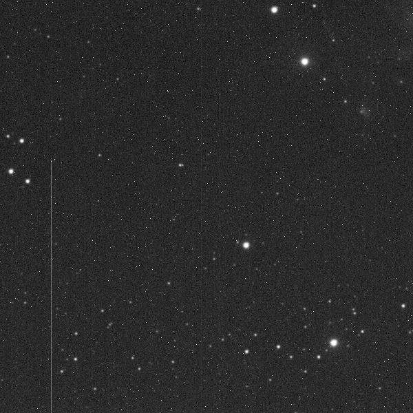
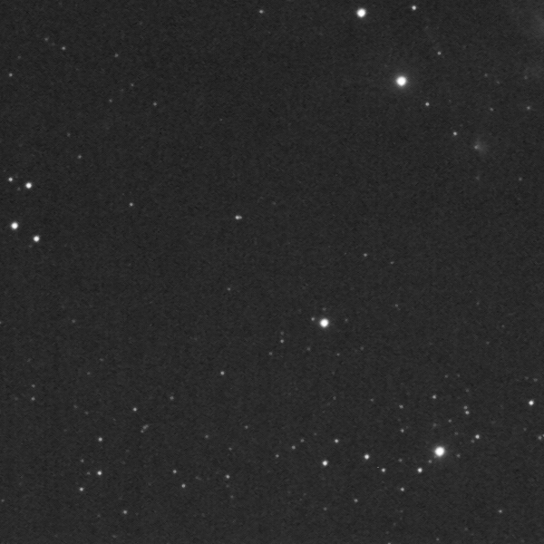
Fix the oversampling: 2×2 binning
Downsample the master
IntegerResampleOPTIONALRight after integration: IntegerResample, Downsample, factor 2, mode Average. The image goes from 3840×2160 at 0.61″/px to 1920×1080 at 1.23″/px.
Imaging without the reducer? See Reducer or native?: at native focal length, 3×3 binning gives about the same 1.2″/px.
When to skip it: on nights of excellent seeing (FWHM under 2″, which you can check in SubframeSelector), on small planetary nebulae where you want maximum scale, or when BlurXTerminator's PSF readout shows stars around 3 px or less.
Linear stage: same steps, different settings
Follow Part B steps 4–9. The differences are:
| Step | MK127 difference |
|---|---|
| Gradients | The 0.65° field is small, so gradients are usually a simple linear ramp. GradientCorrection at defaults is normally enough. Watch for overcorrection around galaxies; turn on structure protection. |
| BXT | Sharpen Stars 0.20–0.30. The Mak's large central obstruction spreads light into bright halos around stars: try Adjust Star Halos −0.05 to 0.00. Sharpen Nonstellar 0.5–0.7 suits small galaxies and planetaries. If a galaxy core has few stars around it, turn off Automatic PSF and set PSF Diameter to the measured FWHM in pixels. |
| SPCC (no filter or UV/IR cut) | QE Ideal QE curve; filters Sony IMX 462-662-585-UVIRCut R/G/B; white reference Average Spiral Galaxy. |
| SPCC (Duo-Band) | Your database has no ZWO Duo-Band entry. Either use SPCC's narrowband mode (H-α 656.3 nm and O III 500.7 nm, with bandwidths from ZWO's spec sheet), or skip SPCC and go to the HOO path below, which assigns colour by palette. |
Worked example: a galaxy (M31, Seestar data)
Gradient correction: keep structure protection on
M31 fills much of the frame, which is exactly the case GradientCorrection's structure protection exists for. In your install it's on by default (threshold 0.10, amount 0.50).


SPCC with the shared Sony curves
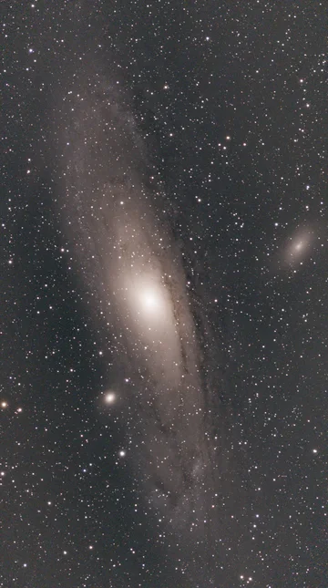
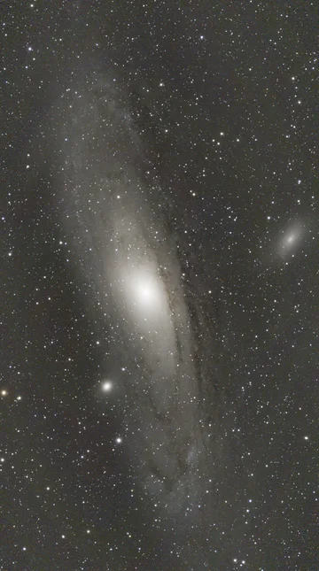
The Seestar's IMX462 and your ASI585MC share one set of curves in the filter database, Sony IMX 462-662-585-UVIRCut R/G/B, so this is the setting you'll use for unfiltered Mak data too. The solve measured 251.7 mm and 2.38″/px.
BlurXTerminator: automatic or manual PSF
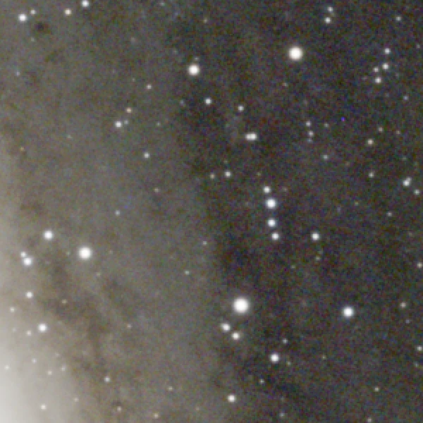
Part C suggests a manual PSF Diameter when a galaxy core has few stars around it. SubframeSelector measured this stack's star FWHM at 2.0 px, so the manual run used PSF Diameter 2.0 with Sharpen Stars 0.25 and Sharpen Nonstellar 0.50.
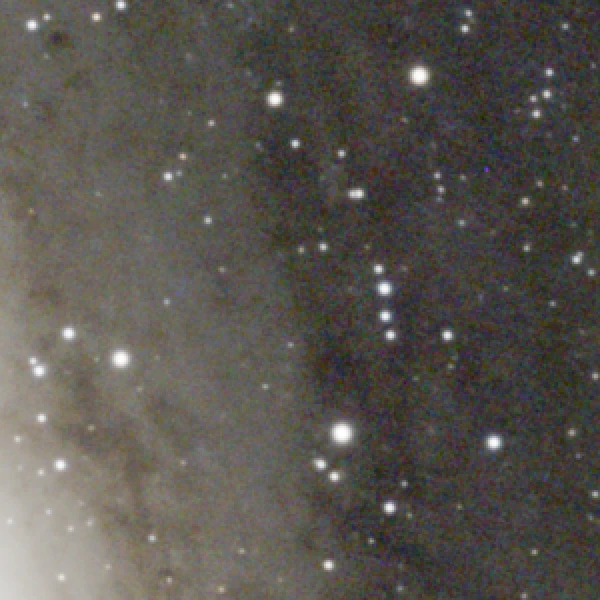
Binning: only when the data is oversampled
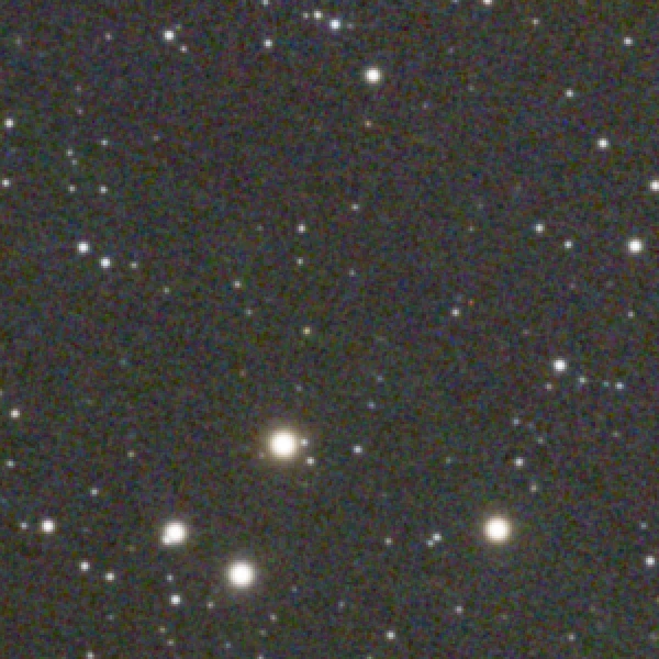
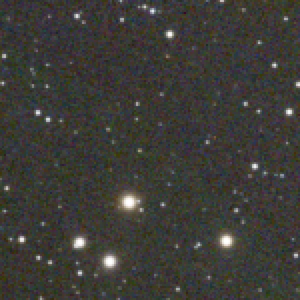
Stretch: no star removal, and protect the core
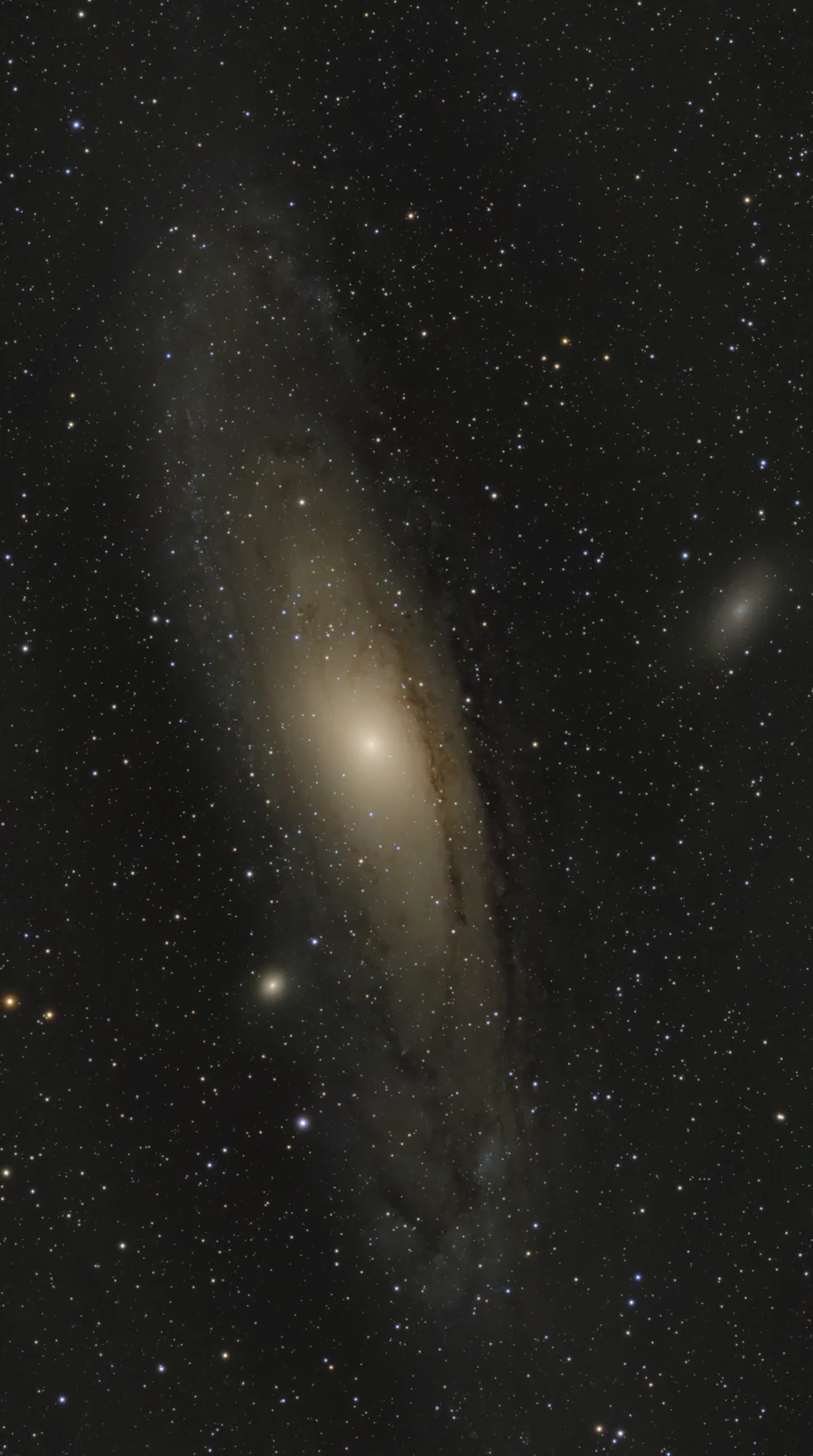
Step 9's note applies: for galaxies, skip StarXTerminator and stretch the whole image. M31's core is far brighter than its disc, so raise MultiscaleAdaptiveStretch's Dynamic range compression.
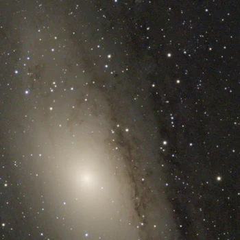
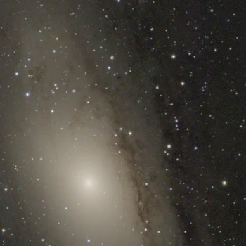
Finish: noise reduction and a masked curve
NoiseXTerminator at 0.60, a gentle global curve to darken the sky (0.15 → 0.11), then a RangeSelection mask (lower limit = background median + 1 σ, fuzziness 0.15, smoothness 6, Lightness on) and a curve through it that adds contrast and saturation (S 0.50 → 0.72) to the galaxy only.
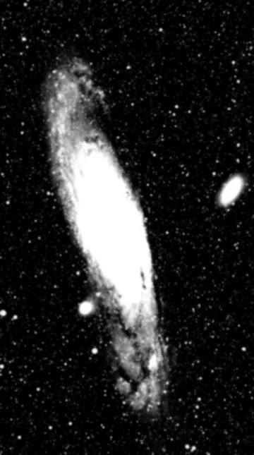
ZWO Duo-Band → HOO palette
With a dual-band filter on a colour sensor, the red pixels record mostly H-α and the green and blue pixels record mostly O III (green and blue both respond near 500 nm). Extracting them gives two narrowband images you can combine into the classic HOO palette: H-α red, O III teal.
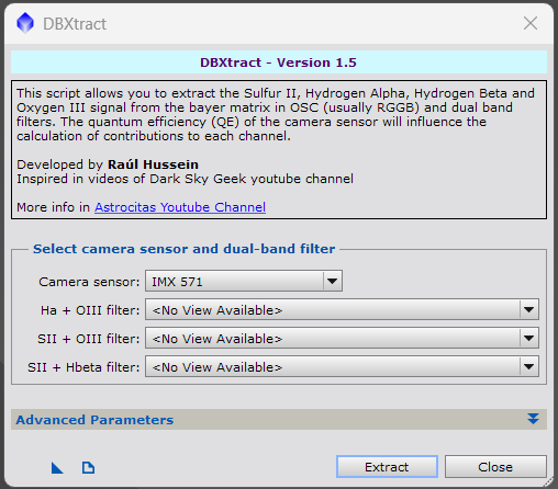
- After gradient correction and BlurXTerminator (still linear), run Script › Suite Astrocitas › DBXtract (installed with your PixInsight). It produces separate H-α and O III images. Script › SetiAstro › NBExtractPI is an alternative.
- Balance the channels. O III is almost always much fainter. Use NarrowbandNormalization or LinearFit to bring the two to a comparable level before combining.
- Combine. In PixelMath with Use a single RGB/K expression unchecked, set R =
Ha, G =OIII, B =OIII, and create a new RGB image. For a richer blend, try G =0.4*Ha + 0.6*OIII. - Continue at Part B step 9 (star removal) and carry on as normal.
For SHO, pseudo-SHO, H-α blends and filter choice, see Appendix D.
Cheat sheet
Printable: three-page version (page 1 processing, narrowband and planets, page 2 sky, angles, time and mosaics, page 3 capture, gear and data) · PDF
| # | Step | Process | Seestar S50 | MK127 + 585MC |
|---|---|---|---|---|
| 1 | Cull | Blink / SubframeSelector | Drop cloud and dew frames | Same; check FWHM for focus drift |
| 2 | Stack | WBPP | Lights only · drizzle only if FWHM < ~2 px · autocrop · solve | Darks + flats + dark flats · no drizzle · solve |
| 3 | Bin | IntegerResample | — | 2× average (optional) |
| 4 | Crop | DynamicCrop | Rotation edges | Dither edges |
| 5 | Gradient | GradientCorrection / GraXpert | Defaults; GraXpert if complex | Defaults; structure protection on galaxies |
| 6 | Correct | BXT Correct Only | ✔ | ✔ |
| 7 | Colour | SPCC | Seestar-LP or IMX462 curves · Ideal QE | IMX585 curves · or Duo-Band → HOO |
| 8 | Sharpen | BXT | Stars 0.25 · halos 0 · nonstellar 0.5 | Stars 0.25 · halos −0.05 · nonstellar 0.6 |
| 9 | Stars out | StarXTerminator | Star image ✔ · Unscreen off on linear data (skip for galaxies) | |
| 10 | Stretch | MAS / ArcsinhStretch | Starless: MAS 0.12–0.15 background · Stars: gentle arcsinh | |
| 11 | Denoise | NoiseXTerminator | 0.7–0.8 | 0.5–0.7 (more integration) |
| 12 | Enhance | Curves / LHE + mask | Gentle S-curve · saturation · LHE 0.2–0.4 | |
| 13 | Recombine | PixelMath | ~((~starless)*(~stars)) | |
| 14 | Export | Save As | XISF master · 16-bit TIFF · sRGB JPEG | |
Histograms at a glance
Background in Appendix A.
| Item | Rule | What to look for |
|---|---|---|
| Value range | 0.0 (black) … 1.0 (white) | Any format; masters are 32-bit float (~7 significant digits) |
| Main peak | Sky background = median | Linear stack: ~0.001–0.005. After stretch: aim 0.10–0.15 |
| Peak width | Noise = MAD | Narrower is smoother; read both in Statistics |
| Right tail | Nebula just right of the peak, stars out to 1.0 | Faint signal sits only a few MADs above the median |
| Spike at 0 | Clipped shadows | Lost data; keep to a tiny fraction of a percent |
| Spike at 1 | Clipped highlights | A few star cores are normal; many means over-stretch or overexposure |
| R, G, B peaks apart | Colour cast | Normal before SPCC; should line up after background neutralisation |
| Linear-only tools | Use values as physics | Gradient removal, SPCC, BXT, rejection |
| Stretched-only tools | Use tonal position | Curves, LHE, saturation, RangeSelection masks |
| STF auto-stretch | black = median − 2.8 × MAD · background → 0.25 | Display only; data stays linear |
| STF linked / unlinked | Linked shows true colour; unlinked hides casts | Judge colour linked, structure either way |
Stretching at a glance
Background in Appendix B; settings in step 10.
| Item | Rule | Note |
|---|---|---|
| Midtones function | MTF(x) = (m − 1)x ÷ ((2m − 1)x − m) | Input m → 0.5 output; m = 0.5 changes nothing; smaller m = harder |
| First stretch | m ≈ 0.005 | Sky 0.002 → 0.285 (×143); star 0.9 → 0.999 (×1.1) |
| Noise | Gain at the background applies to noise too | SNR (integration time) sets how hard you can stretch |
| Black point | Clips everything below it, permanently | Watch clipped-pixel counts in HT |
| Colour | Per-channel curves push bright stars to white | ArcsinhStretch keeps colour ratios |
| Starless | MAS: background 0.15 · aggressiveness 0.7 · DRC 0.4 · contrast recovery on | Faint/short data: 0.22 / 0.9–0.95 / 0.3. Galaxy cores: DRC 0.6 |
| Stars | ArcsinhStretch 10–50, protect highlights; or HT midtones only | Stop when faint stars appear |
| HT | Black, midtones, white once; matches the STF | Quick stretches and small tweaks |
| GHS | Contrast placed at a symmetry point | Staged, precise stretches |
| Strategy | Save linear first · starless and stars separately · two moderate stretches beat one extreme | Check at 1:1 |
| Double-stretch trap | Reset the STF after a permanent stretch | Blown-out look = STF still on |
Arcseconds at a glance
Background and derivations are in Appendix C.
| Rule | Your numbers |
|---|---|
| 1° = 60′ = 3600″ | 1″ = 4.85 µrad · eye resolves ~60″ |
| scale = 206.265 × px(µm) ÷ f(mm) | Seestar 2.39″ · MK127 0.61″ · binned 1.23″ · guider 6.4″ |
| FOV = scale × pixels ÷ 60 | Seestar 76′ × 43′ · MK127 39′ × 22′ |
| FWHM ≈ √(seeing² + diffraction² + guiding² + …) | The largest term dominates |
| Airy FWHM ≈ 1.03 λ/D | Seestar 2.3″ · MK127 0.92″ (550 nm) |
| FWHM(px) = FWHM(″) ÷ scale | Seestar measured ~3 px (7–8″) · MK127 ~3.5–5 px at 2–3″ seeing |
| ideal scale ≈ FWHM ÷ 2…3 | < 2 px: drizzle (Seestar, sharp nights) · > 3 px: bin 2×2 (MK127) |
| FWHM ≈ 2 × HFR | N.I.N.A. HFR to FWHM |
| guiding blur ≈ 2.35 × RMS | Keep RMS ≤ scale ÷ 2: ~0.3″ unbinned, ~0.6″ binned on the Mak |
| sky motion = 15.04″/s × cos δ | Crosses an MK127 pixel in 0.04 s, a Seestar pixel in 0.16 s |
| 1 mas = 0.001″ | Gaia parallax and proper motion units |
Coordinates and units at a glance
Details and worked examples are in Appendix C. A printable three-page version of this whole cheat sheet (Letter, landscape) is also available as a PDF.
| Item | Rule | Example / note |
|---|---|---|
| Angle units | 1° = 60′ = 3600″ | 41° 30′ = 41.5°, not 41.30° |
| DMS → decimal | d + m/60 + s/3600 | 51° 28′ 40.1″ = 51.47781° |
| Decimal → DMS | Remainder × 60 → minutes; remainder × 60 → seconds | 0.47781° × 60 = 28.67′ → 0.67′ × 60 = 40.1″ |
| Signs | N and E positive; S and W negative | The minus applies to the whole value: −0° 30′ = −0.5° |
| RA (time) → angle | 1ʰ = 15° · 1ᵐ = 15′ · 1ˢ = 15″ | M31 RA 00ʰ 42ᵐ 44.3ˢ = 10.6846° |
| RA on the sky | 1ˢ of RA = 15″ × cos(Dec) | At Dec +41°: 11.3″ |
| Dec | Degrees, + north / − south of the celestial equator | M31 Dec +41° 16′ 09″ = +41.2692° |
| FITS headers | RA/DEC decimal degrees; OBJCTRA/OBJCTDEC sexagesimal text | 00 42 44.3, +41 16 09 |
| Ground distance | 1″ latitude ≈ 31 m · 1′ ≈ 1.85 km · 1° ≈ 111 km | Longitude × cos(latitude) |
| Site precision | 2–3 decimal places (≈1 km–110 m) | Enough for GoTo, flips and polar alignment |
| Polar alignment | Polar axis elevation = site latitude | GTi wedge set to your latitude |
| True vs magnetic north | true = magnetic + declination (E +, W −) | Look up magnetic declination (NOAA/NCEI WMM); take compass bearings away from steel |
| UTC and time zones | UTC = local − offset | 21:00 at UTC−5 = 02:00 UTC next day · FITS DATE-OBS is UTC · DST shifts the offset 1 h |
| Sidereal day | 23 h 56 min 4 s | Stars rise ~4 min earlier each night, ~2 h a month |
| Local sidereal time | LST = GMST + longitude ÷ 15 · HA = LST − RA | HA = 0: transit, highest, meridian flip · negative = rising |
| Clock error → pointing | 1 s = 15″ · 1 min = 15′ · 1 h = 15° | Check PC and SynScan time, zone and DST before a session |
| Maximum altitude | 90° − |latitude − Dec| | Reached at transit (HA = 0) |
| Airmass | ≈ 1 ÷ cos(zenith angle) | 45° = 1.41 · 30° = 2.0 · 20° = 2.9 · stay above ~30° |
| Seeing vs altitude | FWHM × airmass0.6 | At 30°: stars ~50% wider |
| Refraction | ≈ 58″ × tan(zenith angle) | 45° = 1′ · 30° = 1.7′ · horizon ≈ 34′ · objects appear higher |
| Dispersion | ≈ 1.5% of refraction (450–650 nm) | 30° = 1.6″ (2.5 Mak px) · blue up, red down · ADC for planets |
| Field rotation (alt-az) | 15.04 × cos lat × cos az ÷ cos alt °/h | Seestar: avoid within ~10° of the zenith |
| Sky brightness | mag/arcsec² (bigger = darker) | 1 mag = 2.512× · 5 mag = 100× · Bortle 8 ≈ 18.0 vs Bortle 2 ≈ 21.9 (36×) |
| Bortle → SQM | 1: 22.0 · 3: 21.7–21.9 · 4: 20.5–21.7 · 5: 19.5–20.5 · 6: 18.9–19.5 · 7: 18.4–18.9 · 8–9: < 18.4 | Approximate; Bortle is visual |
| Integration vs sky | time ∝ sky brightness | Each 1 mag brighter ≈ 2.5× the time (faint broadband targets) |
| Filters | Duo-Band / Seestar LP: emission nebulae in any sky | Galaxies, clusters, M45, dust: filter off, dark site, no Moon |
| Lunar cycle | 29.53 days · rises ~50 min later each day | Broadband window: last quarter → new → first quarter, Moon below the horizon |
| Moon distance | ≥ 60° broadband · ≥ 30° narrowband | Moonlight hurts O III more than H-α |
| Darkness | Sun > 18° below the horizon | Civil 0–6° · nautical 6–12° · astronomical 12–18° · none above ~48.6° latitude at midsummer |
| Polar error → drift | drift ≈ error × 7.29×10⁻⁵ /s | 1° ≈ 0.26″/s · aim ≤ 5′ for the Mak · Polaris is ~37′ off the pole |
| Where the site goes | N.I.N.A. (Options › General › Astrometry), GS Server; Seestar uses the phone's location | Keep N.I.N.A. and the mount in agreement; PixInsight only needs RA/Dec |
Narrowband and filters at a glance
Details, palettes and PixelMath walkthroughs are in Appendix D.
| Item | Rule | Example / note |
|---|---|---|
| Lines | H-α 656.3 · [O III] 500.7 · [S II] 671.6/673.1 · H-β 486.1 nm | S II ≈ 5–20% of H-α · [N II] 658.3 sits inside H-α filters wider than ~3 nm |
| No filter | Galaxies, clusters, reflection and dark nebulae | A narrowband filter removes their starlight |
| Duo-Band / Seestar LP | H II regions, planetaries, SNRs, Wolf-Rayet | Any sky; Moon ≥ 30° away · O III suffers first |
| Broadband LP | Galaxies under old sodium/mercury light | Little help against LEDs · colour cast → SPCC |
| UV/IR cut · IR-pass | Planet colour · planets in poor seeing | ASI585MC window already blocks IR for deep sky |
| HOO | R=Ha · G=OIII · B=OIII | Richer: G = 0.4*Ha + 0.6*OIII |
| Pseudo-SHO | R=Ha · G=0.6*Ha+0.4*OIII · B=OIII | Gold H-α, blue O III without S II |
| SHO | R=SII · G=Ha · B=OIII | Then SCNR green 0.6–1.0 (Average Neutral) → hue curves |
| H-α into RGB | Ha − k(R − med R), k 0.2–0.5 | Add w = 0.5–1 to R, after SPCC · or NBRGBCombination |
| Workflow | Extract (DBXtract) → gradients per channel → stretch each channel separately | No SPCC for SHO · NXT weak channels · RGB stars |
| Integration | H-α : O III : S II ≈ 1 : 2 : 2 | Colour camera: H-α and S II on ¼ of pixels |
| Fast optics | Passband shifts blue: f/2 ≈ 5–9 nm, f/2.8 ≈ half | Use 6–7 nm or high-speed filters on the Samyang 135 |
| Sun | Full-aperture solar film only | Never an eyepiece "sun filter" |
Mosaics at a glance
Planning details per rig are in Appendix C (Seestar, MK127, ASI585MC + 135, R8); processing in Seestar mosaics.
| Item | Rule | Example / note |
|---|---|---|
| Coverage | frame × (N − (N−1) × overlap) | Overlap 15% (ASI585MC, Seestar, Mak) · 20% (R8) |
| Seestar | 0.72° × 1.27° · 2×2 = 1.33° × 2.34° · 3×3 = 1.94° × 3.42° | Each panel gets 1/N of the session · above ~2×2 use the 135 |
| MK127 | 39′ × 22′ · 2×2 = 73′ × 41′ · portrait 3×2 = 60′ × 73′ | ~4 h/panel binned · N.I.N.A. Center every panel |
| ASI585MC + 135 | 4.7° × 2.7° · 2×2 = 8.7° × 4.9° · 3×3 = 12.8° × 7.2° | Heart & Soul 2×1 · Cygnus 3×3 · Orion ~4×4 |
| R8 + 135 / 400 | 15.2° × 10.2° · 2×2 = 27° × 18° / 5.2° × 3.4° · 2×2 = 9.3° × 6.2° | Broadband: dust, Milky Way, galaxies · flats per lens |
| Capture | Same rotation, sub length, gain/ISO and total time per panel | Shoot western panels first · narrowband panels OK under Moon |
| Route A | Solve every sub → MosaicByCoordinates → ImageIntegration (clip low) | Seestar app mosaics and drift · disk = subs × canvas |
| Route B | WBPP per panel (autocrop off) → crop · BXT correct → solve → MosaicByCoordinates → GradientMergeMosaic | Shrink 10 · feather 30 (50–100 on big mosaics) · Mak: bin each panel first |
| Gradients | Per panel if open sky; after merge if nebula fills the panels | MGC + MARS best on the finished mosaic |
| Seams | Fix gradients first, then depth, then feather | Different seeing → BXT correct + cull by FWHM |
| Moon / landscapes | No stars to solve / foreground | Moon: AutoStakkert! → ICE/Hugin · Milky Way: Sequator/SLS → PTGui/Hugin |
Capture and gear at a glance
Details in Appendix E.
| Item | Rule | Example / note |
|---|---|---|
| Sub length | sub ≥ 10 × RN² ÷ sky e⁻/px/s | Mak 30–60 s / Duo 180–300 s · 135 f/2 15–30 s / Duo 60–120 s · Seestar LP on: 20–30 s |
| ASI585MC gain | ~252 (HCG on), default offset | One gain/offset for every rig → one dark library |
| Focus tolerance | ±1.34 × N² µm | 135 f/2 ±5 µm · Mak f/7.7 ±80 µm · refocus each 1–2 °C |
| Polar alignment | TPPA, PHD2 static, SharpCap | Mak < 5′ · 135 < 10′ |
| PHD2 | 3.75 µm, 120 mm → 6.4″/px · 1–2 s · Guiding Assistant | RMS: Mak ≤ 0.3″ (0.6″ binned) · 135 rigs ≤ 2–4″ |
| Dither | In guide pixels | Mak 1–2 · 135 rigs 3–5 · every 1–3 subs |
| Dew | Keep optics 2–3 °C above ambient | Mak shield + strip · lens and guide strips · Seestar heater |
| Power (C300) | ~245 Wh usable | Mak rig ~8–10 h · 135 rig ~9–12 h |
| MK127 | Cool 45–60 min · 55 mm reducer back focus | Solves 955–985 mm · collimate with 3 push-pull pairs |
| Reducer or native | Reducer + 2×2 ≈ native + 3×3 per pixel | Native for planets, Moon, doubles, tiny planetaries |
| Calibration | Darks per exposure in 5 °C bins · flats + dark flats every session | R8: dither + flats · Seestar: lights only |
| Data | Keep lights, masters, project, TIFF | Delete WBPP temp · 3-2-1 backup |
| Comets | Star-register → CometAlignment → two stacks | Sub motion < 1 px |
| Science | Linear, calibrated data only | AAVSO · ETD/ExoClock · IOTA · MPC |
| Export | sRGB → resize → JPEG 90–95 | AnnotateImage for labelled versions |
Troubleshooting
| Symptom | Likely cause | Fix |
|---|---|---|
| Strong green cast after stacking | Normal for OSC sensors: there are two green pixels per Bayer cell | SPCC fixes it. If SPCC failed, check the plate solve, then try again. |
| SPCC: no catalog / no stars matched | Gaia DR3/SP not configured, or a wrong focal length or pixel size in the solve | See setup step 2. Re-solve with 250 mm (Seestar) or your measured Mak focal length. |
| Diagonal streaks ("walking noise") | No dithering; hot pixels and pattern noise line up across frames | Dither in N.I.N.A. For the Seestar, more subs over a longer span help. |
| Dark rings around stars after BXT | Sharpen Stars too high, or halos too negative | Lower Sharpen Stars, raise Adjust Star Halos. |
| Target faded or a dark hole around a galaxy | Gradient overcorrection | Lower GradientCorrection's high threshold, or turn on structure protection. |
| Drizzled image looks noisy or cross-hatched | Drizzle used on data that isn't undersampled (stars ~3 px), or too few subs | Use Scale 1. Drizzle only when SubframeSelector shows stars under ~2 px and you have 200+ subs. BXT Correct Only reduces mild drizzle artifacts. |
| Blotchy, plastic background | Noise reduction too strong | Lower NXT Denoise; accept some grain. |
| Dust donuts survive calibration | Flats shot after focus or rotation changed, or missing dark flats | Reshoot flats without touching the optical train. |
| Mak stars bloated in some subs | Focus drift (mirror moves as it cools) | Cull by FWHM in SubframeSelector; autofocus every 1–2 °C in N.I.N.A. |
Appendix A · Histograms and your image data
Read this appendix first; Appendix B builds on it. A histogram is the most honest view of your data: it shows what the numbers actually are, regardless of how the screen happens to display them.
What a histogram is
A histogram counts pixels by brightness. The horizontal axis is pixel value; the vertical axis is how many pixels have that value. PixInsight normalises every image to the range 0.0 (black) to 1.0 (white), whatever the file format:
| Format | Distinct levels | Where you meet it |
|---|---|---|
| 8-bit integer | 256 | JPEG and your screen |
| 12-bit (IMX462 / IMX585 readout) | 4,096 | Raw sensor ADC; stored in 16-bit FITS |
| 16-bit integer | 65,536 | Subs from N.I.N.A. and the Seestar; TIFF exports |
| 32-bit float | 24-bit precision (about 7 significant digits) at any brightness | Every WBPP master and all processing |
Stacking is why the 32-bit float format matters. Averaging hundreds of 16-bit subs produces values between the original integer levels. That extra precision is real information about faint signal, and only floating point keeps it.
Reading an astro histogram
A deep-sky histogram has a characteristic shape, and each part means something physical:
| Feature | What it is | What it tells you |
|---|---|---|
| The main peak | The sky background: most pixels in a deep-sky image are "empty" sky | Its position is the sky brightness. In PixInsight it's measured as the median. |
| Width of the peak | Random variation of the background: noise | A narrow peak means a smooth background. Measured as MAD (median absolute deviation), a noise estimate that ignores stars. |
| Long tail to the right | Nebulosity, galaxies, then stars | The faint target sits just right of the peak. Stars stretch far out to 1.0. |
| Spike at 0.0 | Clipped shadows | Data crushed to pure black and lost. Normal only in cropped-away edges. |
| Spike at 1.0 | Clipped highlights | Saturated star cores. A few are unavoidable; many means overexposed subs or an over-hard stretch. |
| Separated R, G, B peaks | Colour cast | Before colour calibration this is normal (OSC green, light-pollution orange). After SPCC with background neutralisation, the peaks should line up. |
The linear histogram problem
On linear data, almost the whole image lives in a tiny sliver at the far left. A typical sky background on a stacked master sits around 0.001–0.005. Faint nebulosity might be 0.0005 above that. A bright star core can be 0.9 or more.
Simulated data: 60,000 pixels with a sky background at 0.002, faint nebulosity and a few stars. Both panels are drawn to scale with 128 bins. On the linear side, about 97% of all pixels fall in the very first bin (0 to 0.0078).
That has three practical consequences:
- You can't see it. A screen shows 256 levels. If the useful data spans 0.000 to 0.005, it maps to only the first one or two of those levels: black.
- You can't place controls on it. A curve point, a mask threshold, or a histogram slider would need to sit at something like 0.0023 versus 0.0027. In a histogram widget a few hundred pixels wide, that difference is less than one pixel of mouse travel.
- Histogram-shaping tools misbehave on it. More on that below.
Why some work needs stretched data and some needs linear data
Tools that use your image's statistics fall into two groups, and the difference explains the whole workflow order.
LINEAR Statistics as physics
Gradient correction, SPCC, BlurXTerminator, and pixel rejection during stacking calculate with the actual values: medians, noise estimates, star fluxes. They rely on the values being proportional to light. They don't care that the histogram is squashed, because they read numbers, not a picture.
A stretch would break them. SPCC compares star fluxes with Gaia predictions; after a curve, a star twice as bright is no longer twice the value, so the photometry is meaningless.
NON-LINEAR Histogram as picture
Curves, LocalHistogramEqualization, saturation, and RangeSelection masks change or select data by where it sits in the histogram. They assume the tonal range is spread out so that "shadows", "midtones" and "highlights" each contain meaningful structure.
On linear data, all of the nebula, the sky and its noise share the same few levels in the shadows. These tools can't tell them apart, so they either do nothing visible or amplify noise along with signal.
Some concrete examples:
| Tool | What it does with the histogram | On linear data |
|---|---|---|
| LocalHistogramEqualization | Redistributes values in each neighbourhood so they fill the range more evenly, boosting local contrast | Each neighbourhood is mostly noise around the sky level, so it equalises the noise: a grainy, blotchy mess. |
| RangeSelection masks | Selects pixels between a lower and upper value | Nebula and sky differ by ~0.0005, which is within the noise. The threshold can't separate them cleanly, so the mask is speckled. |
| CurvesTransformation | Remaps values through a curve you draw | All the interesting data lies under the first sliver of the curve. You can't place points accurately there. |
| Saturation boosts | Push colour away from grey | Faint areas have little colour signal relative to noise, so the boost mostly amplifies colour noise. |
The STF: a stretch for your eyes only
The ScreenTransferFunction resolves the conflict. It applies a stretch to what is displayed while the underlying data stays linear. That's why you can see a linear image while running gradient correction and SPCC on it.
STF auto-stretch (the button in the toolbar) does this:
- Measures the median and MAD of each channel.
- Places the black point a little below the background: by default, 2.8 MADs below the median. That clips almost nothing real, but removes the empty range to the left of the peak.
- Picks a midtones value that moves the background to 0.25 on screen.
Those are the same three moves you'll make in a permanent stretch: black point, midtones, and sometimes white point. This is why dragging the STF's settings onto HistogramTransformation reproduces exactly what you see.
Histograms in PixInsight
- HistogramTransformation shows the input histogram on top and a preview of the output below. Use the zoom buttons to magnify the far left so you can actually see a linear peak.
- Statistics (Process › All Processes › Statistics) gives the median, MAD, minimum and maximum of each channel as numbers. It's useful before and after each step.
- GeneralizedHyperbolicStretch has the most informative histogram display, with before and after overlaid, a log scale option, and readouts for the transformed value.
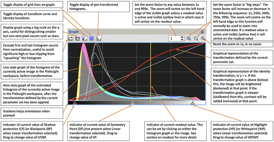
Appendix B · Stretching in depth
Step 10 told you how to stretch. This appendix explains what a stretch is mathematically, why it's needed, what it costs, and how to choose between PixInsight's stretch tools.
Why stretch at all
Your camera and your eyes respond to light in very different ways:
- The sensor is linear. Twice the photons, twice the number, over a huge range. A faint nebula and a 6th-magnitude star can differ in brightness by 10,000× or more, and a 32-bit stack records both.
- Your eyes are roughly logarithmic. You perceive equal ratios of brightness as equal steps, which is why the magnitude scale is logarithmic (each magnitude is a factor of about 2.512).
- The screen has only 256 levels. It cannot show a 10,000:1 range linearly. Either the stars are visible and everything faint is black, or the faint stuff is visible and the stars are pure white over a large area.
A stretch is a non-linear compression of dynamic range. It gives the faint end of the data a much bigger share of the output levels and squeezes the bright end into what's left. It's the astronomical equivalent of what your eye does naturally.
The midtones transfer function
PixInsight's basic stretch, used by HistogramTransformation and the STF, is the midtones transfer function (MTF). For a midtones balance m between 0 and 1:
MTF(x) = (m − 1)·x ÷ ((2m − 1)·x − m)
Its key property: an input value equal to m comes out as exactly 0.5. Set m to your sky background, and the background is lifted to mid-grey. Smaller m means a harder stretch. At m = 0.5 the curve is a straight line and nothing changes.
Curves calculated from the formula above and drawn to scale. The red curve (m = 0.005) is typical of a first stretch on a linear stack.
A worked example
Take three values from a typical linear stack and apply an MTF with m = 0.005:
| Pixel | Linear value | After MTF (m = 0.005) | Change |
|---|---|---|---|
| Sky background | 0.002 | 0.285 | ×143 |
| Faint nebula | 0.004 | 0.444 | ×111 |
| Bright star | 0.900 | 0.999 | ×1.1 |
The nebula was 0.002 above the sky; now it's 0.159 above it, so the contrast between them grew about 80×. Meanwhile, the star barely moved. That asymmetry, huge gain in the shadows and almost none in the highlights, is the whole point of a stretch.
What a stretch costs: noise and clipping
Noise is stretched too
The slope of the curve at any point is its gain there. At the background, the red curve is extremely steep, so every bit of random noise around the sky level is amplified by the same factor as the faint signal. The stretch can't tell them apart.
This is why SNR decides how hard you can stretch. With little integration, the faint nebula is barely above the noise; stretching enough to see it also shows a grainy background. With more hours, the signal grows faster than the noise (√N, see Part A), so the same stretch reveals the nebula with a smoother background. No processing replaces integration time.
Clipping is permanent
Moving the black point right sets every value below it to zero. A little clipping removes the empty range below the sky peak and adds contrast. Too much destroys the faintest signal, which sits just above the background. In HistogramTransformation, watch the clipped-pixel counts: keep shadow clipping to a tiny fraction of a percent.
Moving the white point left saturates everything above it. That's rarely useful for deep-sky images; star cores are already near 1.0.
Colour can shift
Stretching R, G and B separately with the same curve changes the ratios between them. A star that is slightly orange in linear data (R a bit higher than B) gets pushed toward white, because its high values are all compressed toward 1.0. That's why heavily stretched stars look white and why some tools stretch only brightness.
PixInsight's stretch tools compared
| Tool | How it works | Strengths | Use it for |
|---|---|---|---|
| HistogramTransformation (HT) | Black point, midtones (MTF) and white point, applied once | Simple, predictable, matches the STF exactly | Quick stretches; reproducing an STF view; small final tweaks |
| ArcsinhStretch | Inverse hyperbolic sine curve applied to brightness, with the same factor applied to R, G and B | Preserves colour ratios, so stars keep their colour | Stars-only images; colourful targets |
| GeneralizedHyperbolicStretch (GHS) | A family of curves: you choose where contrast goes (symmetry point), how much (stretch factor), and how concentrated (local intensity), with optional shadow and highlight protection | Precise control; can add contrast exactly at the nebula's brightness level | Careful, staged stretches when you want full control |
| MultiscaleAdaptiveStretch (MAS) | Automatic stretch to a target background, with dynamic range compression and multiscale contrast recovery | Reproducible; protects small bright structures and star profiles; good results in one step | The default starless stretch in this guide; HDR targets like M42 |
Practical stretching strategy
- Save the linear image first. A stretch can't be undone, and you'll want to try again later.
- Stretch starless and stars separately (Part B, step 9). The nebula usually needs a hard stretch; stars need a gentle one, or they bloat into white discs.
- Aim the background at 0.10–0.15. The STF's 0.25 looks bright and washed out when printed or shown on a phone. A darker background leaves room for contrast.
- Prefer two moderate stretches to one extreme one when using HT or GHS. Check the histogram between them and stop when the peak is clear of the left edge with no spike at zero.
- Check at 1:1 zoom. A stretch that looks fine when zoomed out often shows background grain or hard-edged faint structures up close.
- Judge with the STF off. After a permanent stretch, reset the STF (or you'll be seeing a stretch on top of a stretch).
Appendix C · Arcseconds: seeing the unit behind every number
Image scale, FWHM, seeing, guiding error and field of view are all measured in arcseconds. This appendix gives you a feel for how small one is, then follows the unit through every stage from the atmosphere to the pixel, using your two rigs.
What an arcsecond is
A full circle is 360 degrees. Each degree is 60 arcminutes (′), and each arcminute is 60 arcseconds (″). So one arcsecond is 1/3600 of a degree, or 1/1,296,000 of a full circle.
A circle is also 2π radians, so one radian is 1,296,000 ÷ 2π = 206,265″. That's the constant in the image-scale formula. For small angles, the angle in arcseconds is simply size ÷ distance × 206,265:
angle (″) ≈ 206,265 × size ÷ distance
The image-scale formula in Your two rigs is the same equation: the "size" is one pixel (µm) and the "distance" is the focal length (mm). The ÷1000 for the unit change turns 206,265 into 206.265.
How small is one arcsecond?
Each object below covers one arcsecond when seen from the stated distance (from the formula above):
| Object | Size | Distance for 1″ |
|---|---|---|
| A human hair | ~70 µm | 14 m: across a tennis court |
| A pencil, end on | 7 mm | 1.4 km |
| A US dime | 17.9 mm | 3.7 km |
| A US quarter | 24.3 mm | 5.0 km |
| A golf ball | 42.7 mm | 8.8 km |
Your unaided eye resolves about 1′ (60″). One Seestar pixel is 1/25 of that, and one MK127 pixel is 1/100 of it.
The diagram below zooms in by 60× twice, from a degree down to an arcsecond. Everything is drawn to scale.
Drawn to scale. Betelgeuse is one of the largest stars in apparent size, and its disc is still 1/14 of an MK127 pixel. Every other star is smaller. The stars in your images are discs only because of blur, which is the subject of the rest of this appendix.
Angular sizes of familiar targets
| Object | Angular size | In Seestar pixels (2.39″) | In MK127 pixels (0.61″) |
|---|---|---|---|
| Andromeda Galaxy, M31 | ~190′ × 60′ | far bigger than the field (mosaic) | far bigger than the field |
| Pleiades, M45 | ~110′ | ~2,760 (mosaic) | ~10,800 (mosaic) |
| Full Moon | ~31′ (1,865″) | ~780 | ~3,040 (wider than the 22′ short side) |
| Orion Nebula, M42 | ~85′ × 60′ | larger than the field | larger than the field |
| Dumbbell Nebula, M27 | ~8′ × 6′ | ~200 × 150 | ~790 × 590 |
| Whirlpool Galaxy, M51 | ~11′ × 7′ | ~280 × 180 | ~1,080 × 690 |
| Ring Nebula, M57 | ~1.4′ × 1′ | ~35 × 25 | ~140 × 100 |
| Jupiter (near opposition) | ~45″ | ~19 | ~73 |
| Saturn's globe | ~18″ | ~8 | ~29 |
| Albireo, separation | ~34″ | ~14 | ~55 |
| Epsilon Lyrae ("Double Double"), each pair | ~2.3″ | ~1 (unresolved) | ~4 |
Your fields of view are 76′ × 43′ (Seestar, 1920 × 1080 px at 2.39″) and 39′ × 22′ (MK127 + 0.65× and ASI585MC, 3840 × 2160 px at 0.61″). The Mak's field is narrower than the full Moon. Field of view is simply image scale × pixel count, ÷ 60 for arcminutes.
Where a star's size comes from
A star is a point, far smaller than any pixel. The disc you see is the sum of several separate blurs, each measured in arcseconds. They add roughly in quadrature (square, add, square-root), so the largest one dominates:
FWHM ≈ √(seeing² + diffraction² + guiding² + focus/optics²)
| Blur source | What it is | Seestar S50 (50 mm) | MK127 (127 mm) |
|---|---|---|---|
| Seeing | Turbulence in the atmosphere; the same for both scopes on a given night | typically 2–4″ | typically 2–4″ |
| Diffraction | Light passing through a finite aperture. FWHM of the Airy disc ≈ 1.03 λ/D (λ = 550 nm). Dawes limit ≈ 116 ÷ D(mm) | 2.3″ (Dawes 2.3″) | 0.92″ (Dawes 0.91″) |
| Guiding / tracking | Mount error during the exposure. A guiding RMS of σ adds about 2.35 σ to the FWHM | alt-az tracking and field rotation; short subs keep it small | PHD2 total RMS 0.8″ ≈ 1.9″ of FWHM |
| Focus, optics, wind | Defocus, temperature drift, aberrations, vibration | varies | varies; refocus as the Mak cools |
| Pixel sampling | Blur from the pixel's own width, small once FWHM ≥ 2 px | significant at 2.39″ | negligible at 0.61″ |
So on a 2.5″ night:
- The MK127 is seeing-limited. Its 0.92″ diffraction disc is small next to 2.5″ seeing. Your guiding is the next biggest term, which is why guiding RMS matters so much on the Mak.
- The Seestar is limited by everything at once. Its 2.3″ diffraction is about the same as the seeing, and its alt-az tracking, short focus and small sensor add more. Your M45 subs measured about 7–8″ FWHM (~3 px) after the soft frames were culled, and the M31 stack about 2 px. That's well above the 3–4″ the formula gives for seeing and diffraction alone.
Pixels per star: sampling
Here is the same patch of sky, 14.4″ square, on each of your sensors, with a star of the stated FWHM centred on a pixel. Each square is one pixel, and its shade is the light that pixel collects. The dashed red circle is the FWHM.
Calculated by integrating a Gaussian star over each pixel and drawn to scale, with a square-root display stretch. Each panel is normalised to its own brightest pixel, so it shows shape, not brightness.
The usual rule of thumb is 2 to 3 pixels across the FWHM, so the ideal image scale is the FWHM ÷ 3 to the FWHM ÷ 2:
| Star FWHM on the night | Ideal image scale | Seestar 2.39″ | MK127 0.61″ | MK127 binned 1.23″ |
|---|---|---|---|---|
| 1.5″ (excellent) | 0.5–0.75″/px | undersampled | ideal | undersampled |
| 2.5″ (good) | 0.83–1.25″/px | undersampled | oversampled | ideal |
| 4″ (average) | 1.33–2.0″/px | slightly undersampled | oversampled | slightly oversampled |
| 7″ (Seestar measured) | 2.3–3.5″/px | ideal | oversampled | oversampled |
This is how to decide for each session. Measure the FWHM in SubframeSelector (below), then check the table. It's also why drizzle helps the Seestar only when its stars are genuinely small, on the best nights with many subs.
Arcseconds per second: how fast the sky moves
The sky turns 360° in one sidereal day (23 h 56 min), which is 15.04″ per second of time at the celestial equator. Further from the equator it's slower, by cos(declination). Without tracking, a star near the equator would cross:
- one MK127 pixel (0.61″) in 0.04 s;
- one Seestar pixel (2.39″) in 0.16 s;
- the MK127's whole 39′ field in about 2.6 minutes.
A 120 s sub on the Mak needs the mount to cancel 1,800″ of sky motion with an error well under 1″, about 1 part in 2,000. That's what PHD2 and the GTi are doing.
Coordinates: degrees, minutes, seconds and decimals
The same 60-based system that gives arcminutes and arcseconds is used for positions on Earth (latitude and longitude) and in the sky (declination). Each value can be written in three ways, and your software uses all of them.
| Notation | Example (Royal Observatory, Greenwich) | Where you meet it |
|---|---|---|
| Degrees, minutes, seconds (DMS) | 51° 28′ 40.1″ N, 0° 00′ 05.3″ W | Star charts, catalogues, mount handsets, Dec in PixInsight dialogs |
| Degrees and decimal minutes (DDM) | 51° 28.668′ N, 0° 00.088′ W | GPS units, some phone apps |
| Decimal degrees (DD) | 51.47781, −0.00147 | N.I.N.A. site settings, FITS headers, web maps, scripts |
Converting
decimal = degrees + minutes ÷ 60 + seconds ÷ 3600
Going the other way: the whole number is the degrees; multiply the remainder by 60 for minutes, and multiply that remainder by 60 for seconds. For 51.47781°: 0.47781 × 60 = 28.6686′, then 0.6686 × 60 = 40.1″, giving 51° 28′ 40.1″.
Signs and hemispheres
- Latitude: north is positive, south is negative.
- Longitude: east is positive, west is negative. That's the convention in N.I.N.A., ASCOM, FITS headers and web maps. A few older tools count west as positive, so check when a GoTo lands on the wrong side of the sky.
- Declination: north of the celestial equator is positive, south negative.
- The sign belongs to the whole value. −0° 30′ is −0.5°, not +0.5°. Values between 0° and −1° are where conversions most often lose the minus sign, as with Greenwich's longitude above.
Right ascension is measured in time
Declination uses degrees, but right ascension (RA) is written in hours, minutes and seconds of time, because the sky turns once a day: 24 h of RA = 360°. So:
| RA unit | Equals (at the celestial equator) |
|---|---|
| 1 hour (1h) | 15° |
| 1 minute of time (1m) | 15′ |
| 1 second of time (1s) | 15″ |
Away from the equator, lines of RA converge toward the pole, so 1s of RA spans 15″ × cos(Dec) of actual sky. At M31's declination (+41°) that's 11.3″; near Polaris it's almost nothing. Don't confuse a second of time in RA with an arcsecond.
Worked example, M31: RA 00h 42m 44.3s, Dec +41° 16′ 09″.
- RA: 0 + 42/60 + 44.3/3600 = 0.71231 h, × 15 = 10.6846°.
- Dec: 41 + 16/60 + 9/3600 = +41.2692°.
FITS headers often carry both forms: RA and DEC in decimal degrees, and OBJCTRA / OBJCTDEC as text such as 00 42 44.3 and +41 16 09. PixInsight's ImageSolver takes RA in hours, minutes and seconds and Dec in degrees, minutes and seconds, or fills them from the header or a Search by object name.
Arcseconds on the ground
One degree of latitude is about 111 km, so one arcminute is about 1.85 km (a nautical mile) and one arcsecond about 31 m. Longitude spans shrink by cos(latitude): at 45° they're about 0.71 of those values.
| Decimal places | Latitude step | Distance (north–south) |
|---|---|---|
| 1 (0.1°) | 6′ | ~11 km |
| 2 (0.01°) | 36″ | ~1.1 km |
| 3 (0.001°) | 3.6″ | ~110 m |
| 4 (0.0001°) | 0.36″ | ~11 m |
For astrophotography, two or three decimal places are plenty. Your site's position only needs to be good to about a kilometre: an error of 1 km shifts where the mount thinks the pole is by about 30″, well under what plate-solved GoTo and PHD2 correct.
Where your site coordinates are used
- N.I.N.A. (Options › General › Astrometry) and the GTi through GS Server use latitude and longitude to convert RA/Dec into where to point, to plan meridian flips and to show altitude. Keep the two in agreement; N.I.N.A. can sync its site to or from the mount.
- Polar alignment: the GTi's polar axis is tilted up by your latitude. The celestial pole sits at an altitude equal to your latitude.
- The Seestar takes its position from your phone's location.
- PixInsight mostly doesn't need the site. Plate solving and SPCC use only RA/Dec. The site matters only for things like computing altitude or atmospheric effects.
True north and magnetic north
An equatorial mount like the GTi has to point its polar axis at the celestial pole, which lies directly above true north. A compass doesn't point there.
| True (geographic) north | Magnetic north | |
|---|---|---|
| Defined by | Earth's rotation axis: the direction along a line of longitude toward the North Pole | Earth's magnetic field, which a compass needle lines up with |
| Relation to the sky | The celestial pole is above it, at an altitude equal to your latitude | None. It's an accident of the planet's molten core |
| Stability | Fixed | Drifts: the magnetic pole moves tens of km a year, and the local offset changes by up to a few tenths of a degree a year |
| Who uses it | Maps, GPS, plate solving, N.I.N.A., your mount's alignment model | Compasses, including a phone compass set to "magnetic" |
The angle between them at your location is the magnetic declination (also called variation). It has nothing to do with the declination of a star. It's measured east (positive) or west (negative) of true north, and across populated areas it ranges from about 0° to 20° or more either way.
true bearing = magnetic bearing + magnetic declination (east positive)
Example: if your declination is 10° W (−10°), a compass reading of 0° is actually 350° true, so true north is 10° to the right of where the needle points. Look up your current value with the NOAA/NCEI magnetic field calculator (World Magnetic Model). It changes over time, so check it every few years.
Why it matters: polar alignment error
A misaligned polar axis makes stars drift in declination and the field slowly rotate. The worst-case drift is about the polar error × the sidereal rate (7.29 × 10⁻⁵ rad/s):
| Polar alignment error | Typical cause | Worst-case drift | Over a 120 s sub |
|---|---|---|---|
| 10° or more | Compass, magnetic declination ignored | ~2.6″/s | ~315″: unusable |
| 2° | Compass, declination applied, metal nearby | ~0.5″/s | ~63″ |
| 0.6° (37′) | Aimed at Polaris itself, not the pole | ~0.16″/s | ~19″ |
| 5′ | Polar scope, or a quick plate-solved alignment | ~0.02″/s | ~2.6″ |
| 1′ | Plate-solved alignment refined (N.I.N.A. TPPA, SharpCap) | ~0.004″/s | ~0.5″ |
PHD2 can correct drift, but every correction is a chance for error, and field rotation can't be guided out at all. For the Mak at 0.61″/px, aim for 5′ or better. So use the compass, with declination applied, only to get the tripod roughly facing north. Set the altitude to your latitude, then refine with the polar scope or a plate-solve routine, which measures the true pole directly from the stars.
The Seestar in its normal alt-az mode doesn't need north at all: it plate solves and tracks in altitude and azimuth. North only matters if you use it on a wedge in equatorial mode, where the same rules apply.
Time zones and sidereal time
Telescopes run on two clocks. Civil time (UTC and your time zone) says when something happened. Sidereal time says which part of the sky is overhead. Mixing them up is behind many GoTo misses and confusing file timestamps.
UTC, time zones and daylight saving
- UTC (Coordinated Universal Time) is the single reference clock. Astronomy software, FITS headers and catalogues use it.
- Your time zone is UTC plus or minus an offset: UTC−5 is five hours behind UTC, UTC+1 one hour ahead. To convert local time to UTC, subtract the offset: 21:00 at UTC−5 is 02:00 UTC the next day.
- Daylight saving time shifts the offset by an hour for part of the year. UTC never changes.
- The date rolls over. Most of a night's session falls on the next UTC date for sites west of Greenwich, and evening sessions start on the previous UTC date for sites far to the east. Files from one night can carry two dates.
| Where | What it uses | Watch for |
|---|---|---|
FITS DATE-OBS | UTC, ISO 8601, e.g. 2026-10-31T03:12:45: the start of the exposure | Not your local time. Your 31 October M45 subs may show 31 Oct or 1 Nov depending on your offset |
| SubframeSelector Site local midnight | The UTC hour of your local midnight | UTC−5 → 5. UTC+1 → 23. Only needed to group frames by night |
| N.I.N.A., GS Server, PHD2 | The mini PC's clock and time zone | Set the PC's time zone correctly and let Windows sync the time. The software converts to UTC itself |
| GTi (SynScan app) | Date, time, time zone and DST you enter or take from the phone | A wrong DST setting is a one-hour error |
| Seestar | Your phone's time and location | Usually automatic |
Sidereal time: the sky's clock
Earth turns once relative to the stars in 23 h 56 min 4 s, a sidereal day. That's about 3 min 56 s shorter than the 24 h solar day, because Earth also moves along its orbit each day. As a result:
- each star rises, transits and sets about 4 minutes earlier every night;
- that adds up to about 2 hours a month, which is why the winter sky has moved into the evening by January;
- the 15.04″ per second sky motion above is 360° per sidereal day, not per 24 h.
Local sidereal time (LST) is the right ascension currently on your meridian, the north–south line through the zenith. It's measured in the same hours as RA, and it ties RA directly to the clock:
hour angle (HA) = LST − RA
| Hour angle | Where the target is | What it means for imaging |
|---|---|---|
| Negative (e.g. −3 h) | East of the meridian, rising | Transit in 3 hours |
| 0 | On the meridian (transit) | Highest in the sky: least air, best seeing and least light pollution. A German equatorial mount like the GTi does its meridian flip here |
| Positive | West of the meridian, setting | Getting lower; plan to finish before it reaches the murk |
LST comes from UTC and longitude. Greenwich sidereal time (GMST) is a formula of the UTC date and time, then:
LST = GMST + longitude ÷ 15 (longitude in degrees, east positive; hours)
Every 15° of longitude is one hour of sidereal time, the same 15°-per-hour rule as RA. You'll rarely compute it yourself: N.I.N.A. shows LST and each target's transit time in the Sky Atlas and Framing Assistant, and the mount computes it from its clock and site.
Worked example, M31 (RA 00h 42.7m) on 15 November 2026: GMST at 00:00 UTC is 3h 36m. M31 transits when LST = 0h 43m:
- at Greenwich (longitude 0°), at about 21:03 UTC;
- at a site at 75° W in UTC−5, LST runs 5 h behind Greenwich, so transit is at about 02:02 UTC, or 21:02 local time;
- a month later, around 19:00 local at either site: about 4 minutes earlier each night.
Sites near the middle of their time zone see a target transit at roughly the same local clock time. Sites near a zone edge are off by up to about 30 minutes, and DST adds an hour.
Clock errors are pointing errors
The mount converts RA to a direction using LST, so a clock error turns directly into a pointing error in RA:
| Clock error | Pointing error (at the celestial equator) | Effect |
|---|---|---|
| 1 s | 15″ | Negligible: plate solving corrects it |
| 1 min | 15′ | Small target near the edge of the Mak's 22′ field |
| 1 h (DST or time-zone mistake) | 15° | GoTo lands in completely the wrong place; alignment stars aren't where expected |
| 12 h (AM/PM mix-up) | 180° | The mount points at the opposite side of the sky |
Plate-solved GoTo in N.I.N.A. hides small errors, but a wrong time zone or DST setting breaks meridian-flip timing and altitude limits, and can send the mount below the horizon. Before a session, check that the mini PC and the SynScan app agree on time, time zone and DST, and sync the PC's clock while it still has internet. Offline in the field, a PC clock can drift by seconds a day.
Altitude, airmass and atmospheric refraction
Every photon you collect has crossed the atmosphere, and the lower the target, the more air it crossed. Altitude affects brightness, sharpness, colour and even where the target appears to be.
Altitude and how high a target gets
Altitude is the angle above the horizon (0° horizon, 90° zenith); azimuth is the compass direction, measured from true north through east. The zenith angle is 90° − altitude. A target reaches its highest altitude when it transits (hour angle 0, see above):
maximum altitude = 90° − |latitude − declination|
At latitude 40° N, M31 (Dec +41.3°) transits 88.7° up, almost overhead, while M42 (Dec −5.4°) only reaches 44.6°. A target whose declination is below latitude − 90° never rises.
Airmass: how much atmosphere
Airmass is the thickness of air along the line of sight, relative to looking straight up. Away from the horizon it's about 1 ÷ cos(zenith angle). The table uses the more accurate Kasten–Young formula, and shows what the extra air does:
| Altitude | Airmass | Seeing (FWHM × airmass0.6) | Extinction, V band (~0.2 mag per airmass) | Refraction | Colour dispersion, 450–650 nm |
|---|---|---|---|---|---|
| 90° | 1.00 | × 1.00 | 0.20 mag | 0 | 0 |
| 60° | 1.15 | × 1.09 | 0.23 mag | 34″ | 0.5″ |
| 45° | 1.41 | × 1.23 | 0.28 mag | 1.0′ | 0.9″ |
| 30° | 2.0 | × 1.51 | 0.40 mag | 1.7′ | 1.6″ |
| 20° | 2.9 | × 1.90 | 0.58 mag | 2.7′ | 2.5″ |
| 10° | 5.6 | × 2.81 | 1.1 mag | 5.4′ | 4.9″ |
| 0° (horizon) | ~38 | — | ~7.6 mag | ~34′ | — |
Airmass from Kasten–Young; refraction from Bennett's formula at standard temperature and pressure; dispersion from the refractive index of air (Edlén). Extinction varies with site and haze; 0.2 mag/airmass is typical of a clear, dark site, and it's larger in blue than in red.
So a target at 30° is seen through twice the air of one overhead. Its stars are about 50% wider for the same seeing (2.5″ becomes ~3.8″), it's 0.2 magnitude dimmer, and it usually sits in the brighter sky glow near the horizon. That's why the 30° rule of thumb exists: below about 30° altitude, the data degrades fast.
Atmospheric refraction
Air bends light downward toward the denser layers, so every object appears higher than it really is. At moderate altitudes the lift is about 58″ × tan(zenith angle). At the horizon it reaches about 34′, more than the Moon's diameter: when the Sun appears to touch the horizon, it's geometrically already below it. Refraction changes by about 1% for every 3 °C of temperature or 10 hPa of pressure.
- Pointing. A mount that ignores refraction misses by up to a few arcminutes at low altitude. Many drivers and planetarium programs have a refraction-correction option; leave it in one place only (driver or software, not both). Plate-solved centring in N.I.N.A. corrects whatever is left.
- Tracking drift. Refraction changes as the target rises or sets, so the target drifts slowly relative to perfect sidereal tracking: tens of arcseconds over an hour at low altitude. Guiding removes it on the Mak; on the Seestar, short subs keep it negligible.
- Field distortion. The bottom of the frame is lifted more than the top, which squashes the field slightly in altitude. Across the Mak's 22′ field, the difference is 0.8″ at 45°, 1.5″ at 30° and 3.2″ at 20°. It changes during the night, which is one reason WBPP's distortion-corrected registration and plate solving with distortion correction help on long sessions and mosaics.
- Polar alignment. Refraction lifts the pole by about 1′ at 45° latitude (more at low latitudes). Plate-solving polar-alignment routines measure the refracted pole, which is close enough for imaging; some offer a refraction option.
Atmospheric dispersion: refraction by colour
Blue light is bent more than red, so at low altitude each star is smeared into a tiny vertical spectrum, blue on top and red underneath. Between 450 and 650 nm the spread is about 1.5% of the refraction: 0.9″ at 45°, 1.6″ at 30°, 2.5″ at 20°.
- Planetary imaging: that's the job of your ZWO ADC (atmospheric dispersion corrector). On the Mak at planetary focal lengths, 1.6″ is many pixels of colour fringing.
- Deep sky with the OSC cameras: at 30° the spread is about 2.5 MK127 pixels (0.61″) but under one Seestar pixel. It shows as blue and red fringes on opposite sides of stars along the vertical. BlurXTerminator's Correct Only pass corrects mild chromatic offsets; the real fix is to image higher.
- Duo-Band data is affected less, because each narrow band is refracted almost uniformly; H-α and O III are just slightly offset from each other, which registration of the extracted channels handles.
Alt-az mounts and the zenith (Seestar)
An alt-az mount like the Seestar's has to rotate the field as it tracks. The rotation rate is:
field rotation (°/h) ≈ 15.04 × cos(latitude) × cos(azimuth) ÷ cos(altitude)
At latitude 40°, due south, that's 13° per hour at 30° altitude, 23°/h at 60°, 66°/h at 80° and 130°/h at 85°. Near the zenith the mount can't keep up, and short subs smear at the corners. Plan Seestar sessions so the target isn't within about 10° of the zenith; for the Seestar, the best part of the sky is roughly 30°–75° altitude. The GTi, being equatorial, has no field rotation and is happy overhead (except around the meridian flip).
Using altitude in practice
- Plan around transit. Centre the session on the target's transit time and stay above ~30°. N.I.N.A.'s Sky Atlas and Framing Assistant plot altitude through the night.
- Read it from the headers. N.I.N.A. writes
CENTALT(altitude) andAIRMASSto each sub. When SubframeSelector shows FWHM rising and star counts falling at the end of a session, check these: it's often altitude, not focus. - Let WBPP's weighting handle the rest. PSF Signal Weight automatically gives low-altitude, softer subs less weight.
Light pollution, sky brightness and the Bortle scale
Sky brightness is measured in magnitudes per square arcsecond (mag/arcsec²): the brightness of one 1″ × 1″ patch of sky, on the same logarithmic scale as star magnitudes. Bigger numbers mean darker skies. A Sky Quality Meter (SQM) reads it directly, and light-pollution maps estimate it from satellite data.
- 1 magnitude = a factor of 2.512 in brightness; 5 magnitudes = exactly 100×.
- A city sky at 18.0 is 100.4 × 3.9 ≈ 36× brighter than a rural sky at 21.9.
- The darkest natural sky is about 22.0. Even there, airglow and starlight set a floor.
The Bortle scale
John Bortle's 9-class scale (2001) describes the sky by what you can see with your eyes. The SQM and naked-eye limiting magnitude (NELM) values below are the commonly quoted approximate equivalents; Bortle is a visual description, so the boundaries are fuzzy.
| Class | Description | SQM (mag/arcsec²) | NELM | What you see |
|---|---|---|---|---|
| 1 | Excellent dark site | 21.99–22.0 | 7.6–8.0 | Zodiacal light, gegenschein and airglow; the Milky Way casts shadows |
| 2 | Truly dark | 21.89–21.99 | 7.1–7.5 | Milky Way highly structured; M33 easy naked-eye |
| 3 | Rural | 21.69–21.89 | 6.6–7.0 | Some glow on the horizon; Milky Way still complex |
| 4 | Rural/suburban transition | 20.49–21.69 | 6.1–6.5 | Light domes over towns; Milky Way visible but washed out near the horizon |
| 5 | Suburban | 19.50–20.49 | 5.6–6.0 | Milky Way faint overhead, gone near the horizon; clouds lit from below |
| 6 | Bright suburban | 18.94–19.50 | 5.1–5.5 | Milky Way only at the zenith, if at all; sky grey-white |
| 7 | Suburban/urban transition | 18.38–18.94 | 4.6–5.0 | Whole sky grey; M31 and M44 barely visible |
| 8 | City | below ~18.38 | 4.1–4.5 | Sky orange or white; only bright constellations |
| 9 | Inner city | below ~18.0 | 4.0 or less | Only the Moon, planets and a few bright stars |
Bortle, J. E. (2001), "Introducing the Bortle Dark-Sky Scale", Sky & Telescope. SQM and NELM ranges are the commonly used approximate mapping.
Sky per pixel: your two rigs
Each pixel sees (image scale)² square arcseconds of sky, so the sky's brightness per pixel depends on the image scale. The rate it fills a pixel per second depends on the focal ratio:
| Seestar (2.39″/px, f/5) | MK127 (0.61″/px, f/7.7) | MK127 binned (1.23″/px) | |
|---|---|---|---|
| Sky area per pixel | 5.7 arcsec² | 0.38 arcsec² | 1.5 arcsec² |
| Per-pixel sky magnitude | SQM − 1.9 | SQM + 1.1 | SQM − 0.4 |
| Sky signal per pixel per second (relative) | 2.4× | 1× | 4× (after binning) |
The faster Seestar fills each pixel with sky glow about 2.4 times as fast as the Mak (that's (7.7 ÷ 5)²). So in the same sky, the Seestar's 10–30 s subs are already sky-limited, while the Mak needs longer subs to swamp its read noise.
What light pollution costs
On a faint target, the dominant noise is the shot noise of the sky glow itself. Noise grows with the square root of the sky brightness, so to reach the same SNR, the required integration time grows in direct proportion to the sky brightness:
time needed ∝ sky brightness → each 1 mag/arcsec² brighter ≈ 2.5× the integration
| Moving from | To | Sky difference | Integration for the same SNR (broadband, faint target) |
|---|---|---|---|
| Bortle 8 (18.0) | Bortle 6 (19.2) | 1.2 mag | ~3× less |
| Bortle 8 (18.0) | Bortle 4 (21.0) | 3.0 mag | ~16× less |
| Bortle 6 (19.2) | Bortle 2 (21.9) | 2.7 mag | ~12× less |
One hour from a Bortle 4 site does roughly the work of two nights in a Bortle 8 city on a faint galaxy. Light pollution also adds the gradients you remove in step 5 and the colour cast SPCC removes in step 7, and it makes noise reduction work harder.
Filters and target choice
- Narrowband and dual-band filters (your ZWO Duo-Band, the Seestar's built-in LP filter) pass only narrow bands around H-α and O III and block most sky glow, including the broad spectrum of white LED lighting. Emission nebulae (M42, Veil, Rosette, North America) image well even in Bortle 7–9.
- They don't help broadband targets. Galaxies, star clusters, reflection nebulae like M45, and dust emit across the whole spectrum, and a dual-band filter throws most of that light away. Image these filter-off, from the darkest site you can reach, and give them more hours.
- Old "LPR" filters cut the narrow sodium lines of older street lights. Modern LED lighting is broad-spectrum, so those filters now do much less.
- The Moon brightens a dark sky by up to about 3 mag/arcsec² at full Moon, turning a Bortle 2 site into roughly Bortle 7 for broadband work. Narrowband tolerates it far better; keep broadband targets for the darker half of the month, and stay well away from the Moon in the sky.
- Altitude matters too: light domes are brightest near the horizon, which is another reason to image above about 30° (see above), ideally on the side of the sky away from the nearest town.
Measuring your own sky
- Maps: lightpollutionmap.info shows modelled zenith brightness (World Atlas) and satellite radiance (VIIRS). Good for choosing sites; it doesn't include the Moon, haze or local lights.
- SQM meter or app: measures the zenith on the night. Readings vary with haze, season and how late it is (many lights go off after midnight).
- Your own subs: with the same rig, filter and exposure, the background median in Statistics is directly proportional to sky brightness. Compare sites or nights by the ratio: a background twice as high is 0.75 mag/arcsec² brighter (2.5 × log₁₀ 2) and needs about twice the integration.
Moon phases and planning a session
The Moon is the brightest light-pollution source most imagers deal with, and it moves on a predictable schedule. Planning around it, together with darkness, altitude and weather, decides more about a night's data than any processing step.
The lunar cycle
The Moon goes from new to new in a synodic month of 29.53 days. It rises on average about 50 minutes later each day (anywhere from about 30 to 70 minutes, depending on season and latitude). Because its phase depends on its angle from the Sun, each phase has typical hours in the sky:
| Phase | Age (days) | Illuminated | Rises / sets (approx.) | Dark sky |
|---|---|---|---|---|
| New | 0 | 0% | Up with the Sun, in daylight | All night |
| Waxing crescent | 3–5 | 10–30% | Sets a few hours after sunset | From late evening |
| First quarter | 7.4 | 50% | Rises ~noon, sets ~midnight | After midnight |
| Waxing gibbous | 10–13 | 70–95% | Sets in the early morning | Only before dawn |
| Full | 14.8 | 100% | Rises at sunset, sets at sunrise | None |
| Waning gibbous | 16–19 | 95–70% | Rises in mid-evening | Early evening only |
| Last quarter | 22.1 | 50% | Rises ~midnight, sets ~noon | Before midnight |
| Waning crescent | 25–27 | 30–10% | Rises a few hours before dawn | Most of the night |
So the useful window for broadband imaging runs from about the last quarter, through new Moon, to about the first quarter: roughly two weeks a month, shrinking at each end as the Moon is up for part of the night. Mean phase dates for the coming weeks (each within about a day; check an almanac or N.I.N.A. for exact times):
| New Moon | First quarter | Full Moon | Last quarter |
|---|---|---|---|
| 9 Nov 2026 | 17 Nov | 24 Nov | 2 Dec |
| 9 Dec 2026 | 16 Dec | 24 Dec | 31 Dec |
Your 31 October M45 subs were shot about 20 days into the cycle, with a waning gibbous Moon roughly three-quarters lit. That didn't matter much for the bright Pleiades stars, but moonlight raises the background and its noise, which is part of why the faint nebulosity needed such a hard stretch (step 10).
How much the Moon matters
- Brightness: a full Moon brightens a dark sky by up to about 3 mag/arcsec² (see above), so broadband data needs roughly 10× the integration time. A thin crescent low in the west costs much less.
- Distance from the target: scattered moonlight falls off with angular distance. Keep at least about 60° from a bright Moon for broadband work and 30° or more for narrowband; closer than that, gradients grow quickly.
- Colour: moonlight is sunlight scattered by the air, so it brightens blue more than red. O III (500.7 nm) suffers more than H-α (656.3 nm); with the Duo-Band near a bright Moon, expect the O III channel to be the noisy one.
- Size: the Moon is 31′ across, wider than the MK127's 22′ short side. For lunar imaging, use mosaics or the Seestar's field.
| Target type | Moon phase that works | Notes |
|---|---|---|
| Galaxies, reflection nebulae (M45), dust, faint clusters | Within ~5 days of new Moon, or with the Moon below the horizon | Broadband, no filter: the Moon is the biggest single factor |
| Emission nebulae with the Duo-Band or Seestar LP filter | Any phase; best away from full | Keep 30°+ away; favour H-α-rich targets when the Moon is bright |
| Bright star clusters, double stars | Any | Moonlight mostly affects the background |
| The Moon itself | Crescent to gibbous | Detail is best along the terminator; a full Moon is flat. The Mak and its 2.25× Barlow suit it |
| Planets | Any | Seeing and altitude matter far more; use the ADC |
Darkness: twilight
The sky isn't fully dark at sunset. Twilight is defined by how far the Sun is below the horizon:
| Twilight | Sun below horizon | For imaging |
|---|---|---|
| Civil | 0–6° | Bright; set up, polar align roughly, focus on a bright star |
| Nautical | 6–12° | Plate solve, start guiding, take flats if you shoot them at dusk; narrowband can start |
| Astronomical | 12–18° | Broadband sky still slightly bright, especially toward the sunset |
| Astronomical darkness | more than 18° | Full darkness: the broadband window |
Near the summer solstice, latitudes above about 48.6° never reach astronomical darkness (the Sun gets no more than 90° − latitude − 23.4° below the horizon at midnight). Narrowband still works then.
Planning a session, step by step
- Pick the dark window. Astronomical darkness, minus the hours the Moon is up (for broadband). N.I.N.A.'s Sky Atlas shows twilight and Moon times for your site.
- Pick a target that's high in that window. Use its transit time (LST = RA, see time) and keep it above 30° (altitude), and at least 60° from a bright Moon. Targets transit about 2 hours earlier each month, so a target that transits around midnight is in season.
- Check the forecast. Cloud, plus transparency (haze) and seeing forecasts, such as Clear Outside, Astrospheric or Meteoblue's astronomy seeing. Transparency matters most for faint broadband targets, seeing most for the Mak at 0.61″/px.
- Choose the filter and sub length. Duo-Band when the Moon is up or the sky is bright; broadband in the dark window. Seestar 10–30 s; Mak 30–60 s unfiltered, 120–300 s with the Duo-Band.
- Plan the meridian flip. On the GTi, note when the target transits and let N.I.N.A. flip a few minutes after.
- Plan focus and calibration. Refocus every 1–2 °C as the Mak cools. Take flats without disturbing the optical train, and make sure your dark library matches the night's gain, exposure and temperature.
- Spread long projects. A faint target needs several dark windows. Shoot it on consecutive moonless nights, or across two new-Moon periods, and stack everything in WBPP, with local normalisation handling the different skies.
Planets with the MK127
Planets are tiny in arcseconds, but bright, which makes them the MK127's strongest targets. Its 127 mm aperture resolves about 0.9″, finer than most nights' seeing, and its long native focal length is made for them. Planetary imaging works differently from deep sky: you record short videos and keep the sharpest frames, so the gear setup and software change too.
Setting up the Mak for planets
| Configuration | Focal length / ratio | Image scale (ASI585MC) | Use it for |
|---|---|---|---|
| 0.65× reducer (deep-sky setup) | ~975 mm, f/7.7 | 0.61″/px | Not for planets: too few pixels across the disc |
| Native, no reducer | ~1500 mm, f/11.8 | 0.40″/px | Poor seeing; the Moon |
| Baader Q-Barlow at 1.3× | ~1950 mm, f/15.4 | 0.31″/px | The usual choice: close to the f/14.5 that suits 2.9 µm pixels |
| Baader Q-Barlow at 2.25× | ~3375 mm, f/26.6 | 0.18″/px | Only excellent seeing (stars under ~1″); otherwise dimmer with no extra detail |
Barlow factors are nominal and change with spacing; measure the real scale from a capture of a double star or of Jupiter's known diameter. The f/14.5 figure is the common lucky-imaging rule of f-ratio ≈ 5 × pixel size in µm.
- Optical train: Mak → ZWO ADC → Q-Barlow → Optolong UV/IR-cut → ZWO ASI585MC. Remove the 0.65× reducer. Use the UV/IR-cut filter to keep infrared from softening the colour image; skip it only if your camera's window already blocks IR.
- ADC: set it for the planet's altitude (see dispersion). Below about 50° altitude it's essential at these scales: at 30° the colour spread is 1.6″, about 5 pixels at 0.31″/px.
- Collimation and cooling: let the Mak cool for 45–60 minutes first; a warm Mak boils the image. Check that a defocused bright star shows concentric rings.
- Mount: the GTi tracks fine for planets. Guiding isn't needed; a region of interest (ROI) a little larger than the planet, with a few re-centres, is enough.
Capture and processing
| Stage | Typical settings | Why |
|---|---|---|
| Capture software | SharpCap or FireCapture (free), writing SER video. N.I.N.A. is built for deep-sky subs, not high-rate video | High frame rates from a small ROI |
| Exposure / gain | 3–15 ms, high gain; histogram peak around 50–70% | Short enough to freeze the seeing |
| Format | RAW8 (bright planets) or RAW16, ROI about 640 × 480 | Debayer later; small ROI = high frame rate |
| Video length | Jupiter ≤ ~3 min; Saturn and Mars up to ~5 min; Venus and Moon unlimited | Jupiter rotates in 9 h 56 min: at 45″, features move 0.9″ (the Mak's resolution) in about 3.5 minutes |
| Stacking | AutoStakkert!: best 5–20% of frames, multiple alignment points | Lucky imaging: keep only the sharpest moments |
| Sharpening | RegiStax wavelets, or PixInsight MultiscaleLinearTransform / deconvolution | Planets need much stronger sharpening than deep sky |
| Derotation (optional) | WinJUPOS | Combines several Jupiter videos into one sharper, lower-noise image |
PixInsight's deep-sky workflow (WBPP, SPCC, BXT and so on) doesn't apply. BlurXTerminator isn't designed for planetary images; use wavelets instead.
What the MK127 shows, and when
Sizes, dates and visibility below were calculated for this guide from standard orbital elements (JPL approximate ephemeris), so dates are good to about a day. Declination tells you how high the planet gets: for northern-hemisphere sites, positive declinations are best.
| Planet | Best window | Size | On the ASI585MC at 0.31″/px | What 127 mm shows |
|---|---|---|---|---|
| Jupiter | Opposition ~11 Feb 2027 (Dec +15°): up all night. Morning sky now; evening from about March | 37″ now; 45″ at opposition | ~145 px | Belts and zones, the Great Red Spot, festoons, the four Galilean moons and their shadows crossing the disc |
| Mars | Opposition ~20 Feb 2027 (Dec +16°). A distant (aphelic) opposition | 7″ now; 13.8″ at opposition; above 10″ from about early January to late March | ~45 px | Polar cap, dark albedo markings (Syrtis Major and others), clouds. Small this time: the next big opposition is 2033 |
| Saturn | Evening sky now, setting earlier each week; behind the Sun around March 2027; opposition ~18 Oct 2027 (Dec +7°) | Globe 19″ now, 20″ at opposition; rings about 2.3× wider | Globe ~65 px | Rings, the globe's shadow on them, Titan and several smaller moons. The rings are still fairly narrow after their 2025 edge-on crossing; the Cassini Division (~0.7″) is at the limit |
| Venus | Morning sky now. Greatest western elongation ~4 Jan 2027 (47°); then a long, low morning apparition through spring | 50″ thin crescent now; 25″ half-lit in January; 10–17″ gibbous by spring | ~80 px at elongation | Phases only; cloud markings need a UV filter. Image in twilight or daylight, when it's higher and the glare is lower |
| Mercury | Morning elongation ~21 Nov 2026 (20° W); evening elongations around 3 Feb and 28 May 2027 | 5–8″ | ~20 px | Its phase. Always low: find it in twilight and use the ADC |
| Uranus | Opposition ~26 Nov 2026 (Dec +21°): well placed all winter | 3.8″ | ~12 px | A small blue-green disc; the brightest moons (Titania, Oberon) with long exposures |
| Neptune | Evening sky now; next opposition ~29 Sep 2027 (Dec +1°) | 2.3″ | ~8 px | A tiny blue disc, and Triton beside it |
Seeing decides everything. Planets don't need a dark sky, so Moon phase and light pollution hardly matter. A steady atmosphere does: watch the Meteoblue or Astrospheric seeing forecast, image when the planet is highest (near transit), and avoid nights after a cold front or under the jet stream. The Seestar can also image planets in its planet mode, but at 2.39″/px Jupiter is only about 19 pixels across.
Double stars with the MK127
Double stars are the purest arcsecond test there is: two points of light a known distance apart. They need no dark sky and little integration, and the MK127 is well suited to them. Its long focal length and 127 mm aperture split pairs close to 1″. Many pairs are true binaries orbiting each other, so their separations and angles slowly change.
How close the MK127 can split
| Limit | Formula | MK127 (550 nm) | What it means |
|---|---|---|---|
| Rayleigh | 1.22 λ/D ≈ 138 ÷ D(mm) | 1.09″ | Each star's peak sits on the other's first dark ring: a clear dip between them |
| Dawes | 116 ÷ D(mm) | 0.91″ | Empirical limit for two equal ~6th-magnitude stars: elongated with a slight notch |
| Sparrow | ≈ 0.95 λ/D | 0.85″ | The dip vanishes; the pair is just an elongated blob. Software can still measure it |
| Seeing | Star FWHM on the night | Usually 1.5–3″ | Usually the real limit. Close pairs need steady nights, short exposures, or both |
Ring and limit values were calculated for this guide from the diffraction pattern of a 127 mm aperture at 550 nm. Blue light splits slightly closer and red slightly wider.
The central obstruction in a Maksutov changes the pattern. Calculated for an obstruction of about a third of the aperture, which is typical of 127 mm Maks:
- The central disc shrinks a little: the first dark ring falls at ~0.98″ instead of 1.09″. This helps with equal pairs.
- About a quarter of the light moves into the first bright ring at ~1.45″, versus 7% with no obstruction. That ring is only about 3 magnitudes fainter than the peak, instead of 4.4.
A faint companion 1–2″ from a bright star sits right on that ring and is easy to miss. Unequal pairs are therefore harder in a Mak than equal pairs at the same separation.
Sampling: which setup for which pair
| Setup | Scale | Pixels across a 1″ pair | Comfortable for pairs wider than |
|---|---|---|---|
| MK127 + Q-Barlow 1.3× (planetary setup) | 0.31″/px | 3.2 | ~1″: the close pairs |
| MK127 native | 0.40″/px | 2.5 | ~1.3″ |
| MK127 + 0.65× (deep-sky setup) | 0.61″/px | 1.6 | ~2″ |
| Seestar S50 | 2.39″/px | 0.4 | ~8″ (its 50 mm aperture resolves ~2.3″, and stars are 7–8″ FWHM) |
Use the planetary setup for anything under ~3″. For it to split cleanly, a pair should be at least about 3 pixels apart and wider than the night's FWHM.
Capturing
- Close pairs (< ~3″): lucky imaging. Use the same SharpCap or FireCapture setup as for planets:
- a small ROI and 1–20 ms exposures;
- gain set so the brighter star peaks around 60–80%, not saturated;
- 1–3 minutes of video.
- Wide pairs (> ~3″): ordinary subs. Take short subs, a few seconds each, at the 0.61″/px deep-sky scale. N.I.N.A. is fine for this. Keep the bright star unsaturated if you want accurate centres.
- Unequal pairs: take two sets of exposures. A short set records the primary unsaturated. A longer set shows the companion; in it, let the primary saturate.
- Colour pairs: use the ADC below ~50° altitude. Otherwise atmospheric dispersion gives each star its own blue and red fringes, and these can be mistaken for, or hide, a companion.
- Altitude and seeing: image near transit. Seeing worse than the separation will merge the pair however well you sample it. A pair that refuses to split on one night may split easily on a steady night.
Measuring separation and position angle
Double stars are described by two numbers:
- separation (ρ), in arcseconds;
- position angle (PA or θ), the direction from the primary to the companion. It's measured from north (0°) through east (90°), south (180°) and west (270°).
Measuring them is a real, publishable kind of amateur science; the Washington Double Star Catalog (WDS) accepts amateur measures. In PixInsight:
- Plate solve the stacked image with ImageSolver. This gives the exact scale and the orientation of north.
- Run DynamicPSF, click both stars, and read their centroid X and Y.
- Calculate the separation: ρ = √(Δx² + Δy²) × scale. Compare it with the catalogue value as a check on your scale.
- Calculate the PA. In an image with north up and east left:
- the companion's north offset is −Δy and its east offset is −Δx, because image y increases downward;
- θ = atan2(east, north), plus 360° if negative, then corrected by the solved rotation angle.
Without a plate solve, use the drift method. Switch off tracking while recording: stars drift west, so the trail direction is PA 270°.
Pairs to try
Separations and magnitudes below are approximate catalogue values. Orbiting pairs (marked ⟳) change by a little each year; check Stelle Doppie (the WDS-based online catalogue) for current figures. The "Season" column assumes northern mid-latitudes, around 9–10 pm local time.
| Pair | Separation | Magnitudes | Season | Why it's worth it |
|---|---|---|---|---|
| Albireo (β Cyg) | 34.7″ | 3.1 / 5.1 | Summer–autumn; low in the west now | Gold and blue: the classic colour pair. Seestar-friendly |
| Almach (γ And) | 9.6″ | 2.3 / 5.0 | Autumn–winter: overhead now | Orange and blue. Seestar can just split it |
| Mesarthim (γ Ari) | 7.5″ | 4.5 / 4.6 | Autumn–winter: now | Matched white twins |
| Achird (η Cas) | 13″ | 3.5 / 7.4 ⟳ | All year (circumpolar); best in autumn | Yellow and reddish |
| Polaris (α UMi) | 18″ | 2.0 / 9.1 | All year | Faint companion close to the bright star; ties in with polar alignment |
| ε Ari | ~1.4″ | 5.2 / 5.5 | Autumn–winter: now | An equal pair near the limit: a good seeing test |
| ζ Aqr | ~2.4″ | 4.3 / 4.5 ⟳ | Autumn; early evening now | Equal pair, slowly widening |
| Rigel (β Ori) | 9.5″ | 0.1 / 6.8 | Winter: from late evening now | The test of glare: a 6.7-magnitude difference |
| Trapezium (θ¹ Ori) | ~9–21″ (four bright stars) | 5–8; E and F 10–11 | Winter | Stars E and F sit within ~4″ of the bright stars, inside the Orion Nebula. A transparency and seeing test |
| Alnitak (ζ Ori) | ~2.3″ | 1.9 / 3.7 | Winter | Bright, close and unequal: a good test of the Mak's first ring |
| 52 Ori | ~1.0″ | 6.0 / 6.1 | Winter | Equal pair at the Dawes limit: the MK127's ceiling |
| β Mon | 7.1″ and 2.8″ | 4.6 / 5.0 / 5.4 | Winter | A fine triple |
| Castor (α Gem) | ~5.5″ | 1.9 / 3.0 ⟳ | Winter–spring | Bright white pair |
| ι Cnc | 30″ | 4.0 / 6.6 | Winter–spring | A "winter Albireo": gold and blue |
| Sirius (α CMa) | ~11″ | −1.5 / 8.4 ⟳ | Winter, at transit | The Pup, a white dwarf, is near its widest. It's only visible on the steadiest nights, in short frames with the primary saturated |
| Algieba (γ Leo) | 4.7″ | 2.4 / 3.6 ⟳ | Spring | Golden pair |
| Mizar (ζ UMa) | 14.4″ | 2.2 / 3.9 | All year; best in spring | With Alcor 12′ away. Seestar-friendly |
| Izar (ε Boo) | 2.9″ | 2.6 / 4.8 | Spring–summer | Orange and blue-green, close and unequal |
| Double Double (ε Lyr) | ~2.2″ and ~2.4″, the pairs 208″ apart | 5.0–6.1 | Summer | Two close pairs in one field: fits the 0.61″/px setup |
- Measured scale: image a wide pair with a well-known separation, such as Mizar, Almach or Albireo, and divide by its separation in pixels. That calibrates the Q-Barlow's real factor (see planets).
- Optics and seeing: splitting ε Ari or 52 Ori tells you your collimation and that night's seeing are both good, before you spend the night on Jupiter.
Deep-sky targets for the Seestar
The Seestar's strength is its wide field: 43′ × 76′ at 2.39″/px, about 1.4 × 2.5 full Moons. Target choice comes down to three numbers:
- Size: does it fit the frame, and is it big enough in pixels?
- Type: should the LP filter be on or off?
- Season: when is it high in the evening?
All three are just arcminutes and hours of RA.
Size: what fits
Target outlines drawn to scale from catalogue sizes and orientations; real nebulae have soft edges that extend further in deep images.
| Target size | On the Seestar (2.39″/px, ~25 px per arcminute) | What to do |
|---|---|---|
| Larger than ~70′ | Overflows the frame | Mosaic mode, or image the brightest part. See Seestar mosaics for processing |
| 20–70′ | 500–1,750 px: fills the frame | The Seestar's sweet spot: large nebulae, big galaxies, clusters |
| 8–20′ | 200–500 px | Good: medium galaxies, small nebulae. Crop in processing |
| 3–8′ | 75–200 px | Recognisable but soft. With stars 7–8″ FWHM (about 3 px), you get shape, not detail |
| Under ~3′ | Under 75 px | Small planetary nebulae and galaxies: a better job for the MK127 at 0.61″/px |
LP filter: on or off
The Seestar's built-in LP filter is a dual-band filter: it passes only narrow bands around H-α and O III.
- On for emission nebulae (H II regions, supernova remnants, planetary nebulae). It cuts sky glow and moonlight while keeping almost all of their light.
- Off for galaxies, star clusters and reflection or dark nebulae. Their light is broadband starlight, and the filter would block most of it.
Use the matching SPCC filter curves for each (step 7).
Season: when it's up in the evening
A target is highest when its RA equals the local sidereal time (see sidereal time). At about 9 pm standard time, mid-month, the sidereal time is roughly:
| Month | Jan | Feb | Mar | Apr | May | Jun | Jul | Aug | Sep | Oct | Nov | Dec |
|---|---|---|---|---|---|---|---|---|---|---|---|---|
| Transiting RA | 4ʰ | 6ʰ | 8ʰ | 10ʰ | 12ʰ | 14ʰ | 16ʰ | 18ʰ | 20ʰ | 22ʰ | 0ʰ | 2ʰ |
The sidereal time advances 2ʰ per month, or 1ʰ per hour of the night. Under daylight saving time, add 1ʰ to the clock time. For a northern site at latitude φ, a target's maximum altitude is 90° − |φ − Dec|. Below about 30° (Dec south of about φ − 60°) seeing, extinction and light pollution all get worse (see altitude).
Targets by season
Sizes are approximate catalogue values for the visible extent. "Best" is the month the target transits around 9 pm; it's well placed for about two months either side. Rows are for northern mid-latitudes.
| Target | Type | Size · Seestar px | Fit | LP | Best | Notes |
|---|---|---|---|---|---|---|
| Autumn–winter: now | ||||||
| M31 Andromeda Galaxy | Galaxy | 178′ × 63′ · 4,470 px long | Mosaic (2–3 panels) | Off | Nov | One frame holds the core with M32 and M110. Bright: 1–2 h gives a good result |
| M33 Triangulum Galaxy | Galaxy | 73′ × 45′ | Tight | Off | Dec | Low surface brightness: 3 h or more, dark moonless sky |
| NGC 869 / 884 Double Cluster | Open clusters | Pair spans ~60′ | Fits | Off | Dec | Both clusters in one frame. 30–60 min; great under moonlight |
| NGC 281 Pacman | Emission | 35′ × 30′ | Fits | On | Nov | Circumpolar from mid-northern sites |
| NGC 7635 Bubble | Emission | 15′ × 8′ · ~380 px | Fits | On | Nov | Shares the field with M52 if framed between them |
| IC 1805 Heart | Emission | ~2.5° | Mosaic | On | Dec | Its core cluster (Melotte 15) region fits one frame |
| NGC 891 | Galaxy | 13′ × 3′ · ~330 × 75 px | Fits (small) | Off | Dec | Edge-on with a dust lane; a test of seeing and focus |
| M45 Pleiades | Cluster + reflection | ~110′ | Mosaic | Off | Jan | Your Part B target. Reflection nebulosity is blue starlight, so the LP filter would remove it |
| NGC 1499 California | Emission | 145′ × 40′ | Mosaic (2 panels) | On | Jan | Faint, nearly pure H-α: 3 h+ |
| M1 Crab | Supernova remnant | 6′ × 4′ · ~150 px | Small | On | Feb | Shape only; filaments need the MK127 |
| M42 / M43 Orion Nebula | Emission | 85′ × 60′ | Core fits; 2 panels for all | On (or off for natural colour) | Feb | Very bright core: the Seestar's 10 s subs help. 30 min already looks good |
| IC 434 / NGC 2024 Horsehead & Flame | Emission + dark | Both within ~50′ | Fits | On | Feb | Frame with Alnitak just off-field; it causes glare. 2 h+ |
| M78 | Reflection | 8′ × 6′ | Fits | Off | Feb | Darker sky needed; dust lanes around it |
| NGC 2237 Rosette | Emission | ~80′ | 1×2 mosaic or tight | On | Feb | Strong O III and H-α: dual-band shines here |
| NGC 2264 Cone & Christmas Tree | Emission + cluster | ~60′ × 40′ | Fits | On | Feb | Fox Fur detail needs 3 h+ |
| M35 (+ NGC 2158) | Open clusters | 28′ | Fits | Off | Feb | A rich cluster with a distant compact one beside it |
| NGC 2359 Thor's Helmet | Emission | 16′ × 8′ | Fits | On | Mar | Dec −13°: low from northern sites; strong O III |
| Spring: galaxy season | ||||||
| M81 + M82 | Galaxies | 27′ and 11′, 38′ apart | Fits | Off | Apr | Circumpolar: possible all year |
| M97 + M108 | Planetary + galaxy | 3′ and 9′, 48′ apart | Fits | Off | Apr | An odd but appealing pair |
| Leo Triplet (M65, M66, NGC 3628) | Galaxies | Group ~45′ | Fits | Off | Apr | A Seestar classic |
| Markarian's Chain | Galaxies | ~90′ | Mostly fits; 2 panels for all | Off | May | A dozen galaxies in one field |
| M51 Whirlpool | Galaxy | 11′ × 7′ · ~275 px | Fits | Off | Jun | Spiral arms visible; best as a close crop |
| M101 Pinwheel | Galaxy | 29′ | Fits | Off | Jun | Low surface brightness: 3 h+ |
| M104 Sombrero | Galaxy | 9′ × 4′ | Small | Off | May | Dec −12°: catch it at transit |
| Summer | ||||||
| M13 | Globular cluster | 20′ | Fits | Off | Jul | Bright; 30–60 min. Short subs keep the core unsaturated |
| M8 Lagoon (+ M20 Trifid, 1.4° north) | Emission | 90′ × 40′ | Mostly fits; mosaic for both | On | Aug | Dec −24°: low from mid-northern sites |
| M16 Eagle / M17 Swan | Emission | 35′ / ~40′ | Fits | On | Aug | Dec −14° / −16° |
| M27 Dumbbell | Planetary | 8′ × 6′ | Small | On | Sep | The Seestar's best planetary nebula: bright with strong O III |
| M57 Ring | Planetary | 1.4′ · ~35 px | Tiny | On | Aug | A ring, but just; one for the MK127 |
| NGC 6888 Crescent | Emission | 18′ × 13′ | Fits | On | Sep | H-α shell with an O III halo in long integrations |
| NGC 6960 / 6992 Veil | Supernova remnant | ~3° loop | Mosaic, or one arc per frame | On | Sep | Each arc fits one frame; fine filaments in H-α and O III |
| NGC 7000 North America | Emission | 120′ × 100′ | Mosaic, or the "Gulf" / Cygnus Wall | On | Sep | Bright H-α; the Wall region fits one frame |
| IC 1396 Elephant's Trunk | Emission | ~170′ | Mosaic, or the Trunk alone | On | Oct | Circumpolar from mid-northern sites |
| NGC 7293 Helix | Planetary | 25′ | Fits | On | Oct | Large but faint; Dec −21°, low from the north |
"Best" months were calculated from each target's RA with the sidereal-time rule above. Integration times are rough guides for a Bortle 5–6 sky and 10 s subs.
- Moonless window: M31, M33, the Double Cluster and NGC 891.
- With the LP filter, under any Moon: the Pacman, Bubble and Heart nebulae.
- Later in the night: M42, the Rosette and the Horsehead rise.
- Field rotation: in alt-az mode, avoid targets passing within about 10° of the zenith (see altitude). Long sessions on one target produce rotated edges that DynamicCrop removes.
- Multiple nights: turn on saving of each frame, and stack sessions together in WBPP. Seeing varies, so cull by FWHM first (step 1).
- Moving up to the MK127: anything under ~8′ (M1, M27, M57, M51, NGC 891) gains real detail at 0.61″/px. Use the Seestar's frame to plan the Mak's 39′ × 22′ crop.
Deep-sky targets for the MK127
The MK127 complements the Seestar. Its field is only 39′ × 22′ at 0.61″/px, about a quarter of the Seestar's area. In return it puts about 4 times as many pixels across each arcminute, and it collects 6.5 times as much light in total. Its targets are the small ones the Seestar renders as smudges:
- galaxies from about 3′ to 25′;
- planetary nebulae;
- globular clusters;
- close-ups of bright parts of large nebulae.
Size: what fits
Each frame is the MK127 + 0.65× + ASI585MC field, 39′ × 22′, north up; shaded = inside, dashed = outside. Outlines are drawn to scale from catalogue sizes. Pixel counts are at the native 0.61″/px (~98 px per arcminute; ~49 when binned 2×2).
| Target size | On the MK127 (0.61″/px) | What to do |
|---|---|---|
| Larger than ~35′ | Overflows the frame | A Seestar target, or image one part of it: a pillar, a wall, an arc |
| 15–35′ | 1,500–3,400 px | Fills the frame. Rotate the camera to line up long targets |
| 3–15′ | 300–1,500 px | The sweet spot: most galaxies, the larger planetary nebulae, globular clusters |
| 1–3′ | 100–300 px | Small planetary nebulae and galaxy groups. Seeing sets the detail |
| Under 1′ | Under 100 px | Bright tiny planetaries: use short subs, or the planetary setup at 0.31″/px (see planets) |
Light per pixel: why binning matters
The signal each pixel gets depends on (aperture × pixel scale)². Both cameras have 2.9 µm pixels, so this is the same as comparing f-ratios.
| Setup | Scale | Light per pixel vs Seestar | Use |
|---|---|---|---|
| Seestar S50, 50 mm f/5 | 2.39″/px | 1× | — |
| MK127 native, 127 mm f/7.7 | 0.61″/px | 0.42× | Bright, small targets: planetary nebulae, globular cores, M42's core |
| MK127 binned 2×2 | 1.23″/px | 1.7× | Faint galaxies and nebulae (see 2×2 binning) |
Two consequences:
- At native scale, the Mak needs about 2.4 times the Seestar's integration for the same per-pixel signal. In return it shows four times finer sampling.
- Binned, it reaches the same depth faster than the Seestar while still sampling twice as finely. With typical 2–3″ seeing (stars 3.5–5 px at native scale), binning loses very little real detail.
Filters and subs
- Emission nebulae and planetary nebulae: ZWO Duo-Band, 120–300 s subs, then the HOO palette. It works under moonlight.
- Galaxies, globular clusters and reflection nebulae: no filter (or only the UV/IR cut), 30–60 s subs, dark moonless nights.
- Galaxies with star-forming regions (M82, M33's NGC 604, M51's arms): adding a few hours of Duo-Band H-α to broadband data brings out red H II regions and M82's red filaments.
- Bright tiny planetaries (NGC 7662, NGC 6543, NGC 7009): 1–10 s subs keep the bright core unsaturated.
- Guiding: PHD2 total RMS ≤ 0.3″ (0.6″ if binning). Dither every 1–3 subs. Refocus every 1–2 °C (see capture habits).
Targets by season
"Best" is the month the target transits around 9 pm (see the RA-by-month table in Seestar targets). Sizes are approximate catalogue values. Southern declinations are low from northern mid-latitudes. Duo = ZWO Duo-Band; none = no filter or UV/IR cut only.
| Target | Type | Size · MK127 px | Filter | Best | Notes |
|---|---|---|---|---|---|
| Autumn–winter: now | |||||
| NGC 7331 + Stephan's Quintet | Galaxy + group | 10′ × 4′ · ~1,000 px; Quintet ~3′, 30′ away | None | Oct | Both fit corner to corner (the diagonal is 45′). The Quintet's galaxies are 13–14 mag: 4 h+, binned |
| NGC 7662 Blue Snowball | Planetary | ~0.5′ · ~50 px | Duo or none | Nov | Bright and tiny: short subs, or planetary setup |
| NGC 7635 Bubble | Emission | 15′ × 8′; bubble ~3′ | Duo | Nov | The bubble shell finally shows structure; strong O III |
| NGC 891 | Galaxy | 13′ × 3′ · ~1,300 × 250 px | None | Dec | Edge-on with its dust lane resolved. Rotate the camera to lay it along the frame |
| M74 | Galaxy | 10′ · ~1,000 px | None | Dec | Face-on spiral with very low surface brightness: binned, 5 h+, darkest sky |
| M77 | Galaxy | 7′ × 6′ | None | Dec | Bright core, faint outer ring |
| M76 Little Dumbbell | Planetary | 2.7′ × 1.8′ · ~270 px | Duo | Dec | Faint outer loops in long O III |
| M33 core / NGC 604 | Galaxy / H II region | Core region fills the frame; NGC 604 ~1.5′ | None + Duo | Dec | NGC 604 is a star-forming region 2.7 million light-years away, resolved as a nebula |
| M1 Crab | Supernova remnant | 6′ × 4′ · ~600 px | Duo | Feb | Filaments show. A Mak classic |
| M42 core and Trapezium | Emission | Core ~20′: fills the frame | Duo or none | Feb | Expose for the core with 5–15 s subs and the rest with longer subs, then blend (HDRComposition) |
| Horsehead (Barnard 33) | Dark on emission | ~8′ × 6′ head, in IC 434 | Duo | Feb | Frame the head and the edge of IC 434; Alnitak just out of field. 4 h+ |
| M78 | Reflection | 8′ × 6′ | None | Feb | Dust lanes around a blue glow |
| NGC 2261 Hubble's Variable Nebula | Reflection | ~2′ × 1′ · ~200 px | None | Feb | Changes shape over weeks as shadows move across it: image it monthly |
| Cone Nebula | Emission + dark | ~10′ region | Duo | Feb | Close-up of the Seestar's NGC 2264 field |
| NGC 2359 Thor's Helmet | Emission | 16′ × 8′ | Duo | Mar | Fills the frame; strong O III. Dec −13° |
| NGC 2392 Eskimo | Planetary | ~0.8′ · ~80 px | Duo or none | Mar | Bright and tiny: short subs |
| Spring: galaxy season | |||||
| M81 | Galaxy | 27′ × 14′ | None | Apr | Rotate the camera so its long axis runs along the frame; spiral arms resolved. Circumpolar |
| M82 | Galaxy | 11′ × 5′ | None + Duo | Apr | Add H-α for its red outflow filaments |
| NGC 2903 | Galaxy | 12′ × 6′ | None | Apr | Bright barred spiral, overlooked |
| M65 + M66 | Galaxies | ~10′ each, 20′ apart | None | Apr | Two of the Leo Triplet (NGC 3628 needs the Seestar or 2 panels) |
| M97 Owl | Planetary | 3.4′ · ~330 px | Duo | Apr | The "eyes" need good seeing and O III depth |
| M106 | Galaxy | 19′ × 8′ | None + Duo | May | Anomalous red arms in H-α |
| M64 Black Eye | Galaxy | 10′ × 5′ | None | May | Dark dust band over a bright core |
| M63 Sunflower | Galaxy | 12′ × 7′ | None | May | Flocculent arms resolve into knots |
| M104 Sombrero | Galaxy | 9′ × 4′ · ~880 px | None | May | Dust lane crisp at this scale. Dec −12°: image at transit |
| NGC 4565 Needle | Galaxy | 16′ × 3′ | None | May | Edge-on, laid along the frame's long side |
| M51 Whirlpool | Galaxy pair | 11′ × 7′ · ~1,100 px | None + Duo | Jun | The showpiece: arms, dust, the bridge to NGC 5195, pink H II knots |
| M101 Pinwheel | Galaxy | 29′ × 27′ | None | Jun | Taller than the frame: crop or 2 panels. Very faint arms: bin, 6 h+ |
| M3, M13 | Globular clusters | 18′, 20′ | None | Jun, Jul | Resolved nearly to the core. 30–60 s subs; 1–2 h. M13's companion galaxy NGC 6207 is 28′ away and fits in the frame |
| Summer | |||||
| NGC 6543 Cat's Eye | Planetary | ~20″ core · ~35 px | Duo or none | Aug | Very bright core in short subs; faint outer halo (~5′) in long Duo-Band |
| M57 Ring | Planetary | 1.4′ × 1′ · ~140 px | Duo | Aug | The ring's structure, central star and faint outer halo. Galaxy IC 1296 sits 4′ away |
| M16 Pillars of Creation | Emission | Pillars ~4′ in a 7′ core | Duo | Aug | Dec −14°: low, so pick steady nights |
| M17 Swan, M20 Trifid | Emission | ~11′ bright core; 28′ | Duo (M20: none for the blue half) | Aug | Low from northern sites; M20 just fits diagonally |
| M27 Dumbbell | Planetary | 8′ × 6′ · ~800 px | Duo | Sep | The "apple core" and its faint outer shell |
| NGC 6888 Crescent | Emission | 18′ × 13′ | Duo | Sep | Fills the frame; braided H-α filaments |
| Pickering's Triangle (Veil) | Supernova remnant | ~30′ section | Duo | Sep | Fine filaments at full resolution |
| Cygnus Wall (NGC 7000) | Emission | A 39′ strip | Duo | Sep | The ridge of the North America Nebula |
| NGC 7009 Saturn Nebula | Planetary | ~0.5′ with its "rings" | Duo or none | Sep | Bright and tiny: short subs |
| NGC 7023 Iris | Reflection | 18′ | None | Sep | Blue petals with brown dust: dark sky, 5 h+ |
| Elephant's Trunk (vdB 142) | Emission + dark | Trunk ~20′ | Duo | Oct | Close-up of the Seestar's IC 1396 field |
"Best" months were calculated from each target's RA with the sidereal-time rule. Integration times are rough guides for a Bortle 5–6 sky with the GTi guided.
- Moonless window: NGC 891, NGC 7331 and M77, binned.
- Under any Moon: the Bubble, M76 and NGC 7662 with the Duo-Band.
- After midnight: M1, then M42's core.
- Pair the rigs: image a region wide with the Seestar, and use that frame to plan the Mak's close-up. The Mak's field covers about a quarter of the Seestar's, so mark it on the Seestar image to choose the framing.
- Camera rotation: set it before you start, from a plate solve in N.I.N.A.'s framing assistant, and keep it for every session on that target so the data stacks without wasted edges.
- Watch the GTi: long subs at 0.61″/px expose guiding errors that the Seestar never shows. Check eccentricity in SubframeSelector (step 1) and cull elongated subs.
Deep-sky targets for the Canon R8
The R8 fills the gap above the Seestar: fields from 5° to 100° across, which neither telescope can reach. It has a full-frame 6000 × 4000 sensor with large 5.98 µm pixels. With your lenses it covers constellations, the Milky Way, and big nebula complexes that are mosaics on the Seestar. On the GTi with the Samyang 135 mm f/2, it collects light per unit of sky about six times faster than the Seestar's f/5.
Lenses, scale and field
| Lens on the R8 | Scale | Field | Untracked limit (NPF) | Best for |
|---|---|---|---|---|
| Laowa 15 mm f/2 (at f/2.8) | 82″/px | 100° × 77° | ~17 s at f/2 (~19 s at f/2.8) | Milky Way landscapes, meteor showers, aurora, zodiacal light |
| RF 24–50 mm (24 mm f/4.5) | 51″/px | 74° × 53° | ~14 s | Constellations, Milky Way panoramas |
| RF 24–50 mm (50 mm f/6.3) | 25″/px | 40° × 27° | ~8 s | Orion with Barnard's Loop, Cygnus, Taurus with the Hyades and Pleiades |
| Samyang 135 mm f/2 (at f/2.8) | 9.1″/px | 15.2° × 10.2° | ~2 s: track it | The deep-sky workhorse: nebula complexes, M31, Orion's belt and sword |
| RF 100–400 mm (400 mm f/8) | 3.1″/px | 5.2° × 3.4° | ~1 s: track and guide | All of M31, the Veil, California, Rosette with the Cone |
| RF-S 55–210 mm (210 mm f/6.3, crop mode) | 5.9″/px | 6.1° × 4.1° | ~2 s | Works, but slow and only 9 MP: the 135 or 400 are better |
Scale = 206.265 × 5.98 µm ÷ focal length; field from the 36 × 24 mm sensor. The untracked limit uses the simplified NPF rule, t ≈ (35 N + 30 p) ÷ f, for pinpoint stars. The old "500 rule" allows about twice as long, but with visible trails at 6 µm pixels.
All three rigs together give a zoom ladder: the 135 mm frame holds about 170 Seestar frames, and the Seestar frame holds about 4 MK127 frames. A typical plan:
- Frame a region with the R8.
- Pick a nebula from it for the Seestar.
- Pick a detail from that for the Mak.
What's different about the R8
- It's not astro-modified. The stock filter in front of the sensor passes only a fraction of H-α (656 nm), commonly quoted as around 20–30%. Red emission nebulae (Barnard's Loop, California, the Heart) come out faint and pinkish, though long integration still shows them. Blue reflection nebulae, galaxies, star fields and the Milky Way are unaffected.
- Filters:
- The Samyang 135 is an EF-mount lens, so it works with your Canon drop-in adapter and its astro LP filter. Use the filter for emission nebulae in light-polluted skies; take it out for galaxies and the Milky Way.
- The RF lenses can't use the drop-in adapter. They need front-thread filters, if any.
- Capture settings:
- RAW (CR3), manual focus at 10× magnified live view on a bright star (a Bahtinov mask helps);
- ISO 800–1600;
- long-exposure noise reduction off (it doubles the time; use dithering and darks instead);
- lens stabilisation off on a tracker;
- electronic first curtain on.
- Stop down a little: f/2.8 on the 135 mm and the 15 mm fixes most corner coma and vignetting for a small loss of speed.
- Tracking:
- The R8 with the Samyang 135 weighs about 1.3 kg, well within the GTi's 5 kg capacity, mounted on a ball head or dovetail.
- At 9.1″/px, unguided 60–120 s subs work with good polar alignment: a 5′ error drifts only about 0.02″/s (see north).
- At 400 mm, guide with the UniGuide.
- Temperature: the sensor has no cooling, so take darks at the session's temperature (or rely on dithering), and flats for every lens and aperture. Flats matter most here: wide lenses vignette strongly.
Processing differences in PixInsight
- WBPP reads CR3 files directly. The Canon Bayer pattern is RGGB, and WBPP normally detects it.
- Wide lenses distort the star field. At 50 mm and shorter, turn on Distortion correction in WBPP's registration settings (StarAlignment). Otherwise the corners won't align and stars will double.
- Gradients are huge over 15–40° fields, with light domes and airglow. Use MultiscaleGradientCorrection or GraXpert carefully, and mask out landscape foregrounds.
- SPCC works the same way; use a generic DSLR or Ideal QE sensor curve unless an R8 curve is listed.
- For landscapes, the sky and foreground need separate stacks: track the sky and take one untracked frame for the ground.
Targets by season
"Best" is the month the target is high around 9 pm. Sizes are approximate. The "LP filter" column applies to the Samyang 135 with the drop-in adapter.
| Target | Size | Lens | LP filter | Best | Notes |
|---|---|---|---|---|---|
| Autumn–winter: now | |||||
| M31 with M32, M110 | 3° × 1° | 135 mm or 400 mm | Off | Nov | The 400 mm frames it like the Seestar's 3-panel mosaic in one shot |
| M31 + M33 region | 15° apart | 50 mm | Off | Nov | Two Local Group galaxies in one frame |
| Double Cluster + Heart & Soul | ~7° span | 135 mm | On | Dec | Clusters and nebulae together; the nebulae are faint on a stock camera |
| M45 + California | ~13° apart | 135 mm (diagonal) | Off | Jan | Blue reflection nebula and red emission in one frame; dark sky needed. In very dark skies, faint dust (Taurus molecular clouds) surrounds both |
| Taurus: Hyades, Pleiades, Aldebaran | ~20° | 50 mm | Off | Jan | Star colour and two open clusters |
| Orion's belt and sword | ~8° | 135 mm | Off or on | Feb | M42, Running Man, Horsehead, Flame and M78 in one frame |
| Orion with Barnard's Loop | ~25° | 24–50 mm | Off | Feb | The loop is faint pure H-α: hard on a stock R8; several hours, dark sky |
| Rosette + Cone (NGC 2264) | ~5° apart | 135 mm | On | Feb | Both nebulae plus open clusters |
| Winter Milky Way (Cassiopeia to Orion) | ~90° | 15 mm | Off | Dec–Feb | Fainter than the summer core, but rich in clusters |
| Geminids meteor shower | Whole sky | 15 mm | Off | Peak night 13–14 Dec 2026 | Moon is a thin evening crescent (new 9 Dec): an excellent year. Hundreds of 15–20 s frames; keep those with meteors and composite |
| Spring | |||||
| Virgo Cluster with Markarian's Chain | ~8° | 135 mm | Off | May | Dozens of galaxies as small smudges; crop for Markarian's Chain |
| Leo Triplet + M95/M96/M105 | ~8° span | 135 mm | Off | Apr | Two galaxy groups in one field |
| M81/M82 region | ~1° pair | 400 mm | Off | Apr | The dust around them (integrated flux nebula) needs a very dark site |
| Rho Ophiuchi complex | ~5° | 135 mm | Off | Jun | Colourful clouds around Antares. Dec −24°: low from the north, so catch it at transit |
| Summer | |||||
| Milky Way core | ~30° | 15–24 mm | Off | Jun–Aug (spring mornings) | The classic landscape target. Low from the north: find a dark southern horizon |
| Lagoon + Trifid (M8, M20) | 1.5° apart | 135–400 mm | On | Aug | Low (Dec −24°); M20's blue half shows well on a stock camera |
| Cygnus: Sadr region, Butterfly, Crescent | ~10° | 135 mm | On | Sep | Rich H-α region, still impressive on a stock camera with long integration |
| North America + Pelican | ~3° | 135–400 mm | On | Sep | The brightest big H-α target for an unmodified camera |
| Veil complex | ~3° loop | 400 mm | On | Sep | The whole loop in one frame |
| IC 1396 Elephant's Trunk region | ~3° | 135–400 mm | On | Oct | Single frame instead of a Seestar mosaic |
Field widths and separations are approximate. Geminid peak date from its usual 13–14 December maximum; Moon phase from the Moon section.
- On the GTi with the 135 mm: M31, then the Double Cluster, then the Pleiades with the California Nebula.
- Later: Orion's belt and sword.
- On a tripod with the 15 mm: the winter Milky Way, and then the Geminids on 13–14 December.
The R8 on the MK127? It's possible, but it would need an RF T-ring, which isn't in your kit. With the 0.65× reducer it would give 1.27″/px over 2.1° × 1.4°, close to the ASI585MC's binned scale over a larger field. The ASI585MC is still the better match there. It's lighter and records H-α fully, and N.I.N.A. controls it more easily.
Targets for the Samyang 135 on the ASI585MC
The ZWO EOS-T2 adapter lets the ASI585MC use the Samyang 135 mm f/2, an EF-mount lens; the Rokinon 135 is the same optical design. This gives a fourth rig, between the R8 and the Seestar:
- Field: 4.7° × 2.7°, at 4.43″/px.
- Speed: at f/2 it gathers light per unit of sky 6.25 times faster than the Seestar.
- H-α: unlike the stock R8, it records H-α fully.
Big emission nebulae that are mosaics on the Seestar and faint on the R8 fit one frame here.
How it compares
| Rig | Scale | Field | Light per pixel vs Seestar | H-α |
|---|---|---|---|---|
| Seestar S50 | 2.39″/px | 0.7° × 1.3° | 1× | Full |
| ASI585MC + Samyang 135 f/2 | 4.43″/px | 4.7° × 2.7° (14 Seestar fields) | 6.3× (3.2× at f/2.8) | Full |
| R8 + Samyang 135 f/2.8 | 9.1″/px | 15.2° × 10.2° | 13.6×, but its larger pixels each cover 4.3× more sky | Weak (stock filter) |
| R8 + RF 100–400 at 400 mm f/8 | 3.1″/px | 5.2° × 3.4° | 1.7×; per area of sky, 8× slower than the 135 at f/2.8 | Weak |
Scale = 206.265 × 2.9 µm ÷ 135 mm; field from 3840 × 2160 px. Light per pixel ∝ (aperture × scale)², which for equal pixel sizes reduces to (f-ratio)⁻².
Frames are 4.73° × 2.66°, north up; outlines drawn to scale from catalogue sizes and positions. Red = emission nebula, teal = galaxy.
Setting it up
- Back focus: EF lenses focus at 44 mm from the sensor. ZWO's EOS-T2 adapter is made to give this with ZWO cameras when you use the spacers its instructions call for. If you can't reach infinity focus, or stars in the corners are stretched, the spacing is wrong.
- Aperture: the ASI585MC's 12.8 mm diagonal uses only the sharp centre of a lens designed for full frame. Corner coma and vignetting, the R8's reasons to stop down, mostly disappear. Start at f/2. Close to f/2.4–2.8 only if bright stars show blue or violet halos (residual colour error).
- Focus: the lens focuses past infinity, so don't trust the hard stop. Focus with a Bahtinov mask or N.I.N.A.'s HFR readout, then tape the ring. At f/2 the critical focus zone is only about ±5 µm (±10 µm at f/2.8), so refocus when the temperature drops a few degrees.
- Filters:
- The camera's window already blocks IR, so no UV/IR-cut filter is needed.
- For emission nebulae, use the ZWO Duo-Band, at least as fast as f/2.8. Narrowband filters shift slightly toward blue at very fast f-ratios, which costs some signal at f/2.
- Check whether your EOS-T2 adapter has a filter thread inside. If it does, the 2″ Duo-Band screws in there, close to the sensor; otherwise it needs a 77 mm front-filter step-up arrangement.
- Mounting and guiding:
- Lens and camera weigh about 1 kg. Carry them on the GTi with a lens ring or dovetail, plus the UniGuide.
- At 4.43″/px the guiding is forgiving. The guide scale (6.4″/px) is close to the imaging scale, and PHD2 total RMS under ~2″ is plenty.
- 60–120 s subs often work unguided with a good polar alignment.
- Subs:
- Broadband: 15–60 s at f/2, because the sky background fills quickly.
- Duo-Band: 60–180 s.
- Keep the same gain and offset as your Mak sessions, so one bias and dark library serves both, with darks for each new exposure length.
- Calibration: darks, flats and dark flats, exactly as for the Mak (see calibration library). Retake flats whenever you change the aperture or remove the camera from the lens.
Processing
Use the MK127 workflow (Part C) with three changes:
- No binning: 4.43″/px isn't oversampled. Stars are typically 2–3 px FWHM, so on sharp nights drizzle ×2 can help (see sampling).
- Plate solving: set focal length 135 mm and pixel size 2.9 µm in WBPP and ImageSolver.
- Gradients: a 4.7° field picks up stronger gradients than the Mak's 0.6°; GradientCorrection or MGC matters more.
SPCC uses the same IMX585 curves, with the Duo-Band settings for HOO.
Targets by season
Targets chosen to fill the 4.7° × 2.7° frame. "Best" is the month the target transits around 9 pm (see the RA-by-month table). Duo = ZWO Duo-Band; none = no filter. Rotate the camera to fit long targets.
| Target | Size · px | Filter | Best | Notes |
|---|---|---|---|---|
| Autumn–winter: now | ||||
| M31 with M32, M110 | 3° × 1° · ~2,500 px long | None | Nov | The whole galaxy and its halo in one frame. 2–3 h at f/2 goes deep |
| Bubble + M52 + Cave Nebula | ~1.5° group | Duo | Nov | A cluster and two nebulae in one field |
| M33 | 73′ × 45′ · ~990 px | None | Dec | Small in the frame, but faint outer arms show quickly at f/2 |
| Heart (IC 1805) or Soul (IC 1848) | ~2.5° each, ~2.7° apart | Duo | Dec | One per frame; both in a 2-panel mosaic (N.I.N.A. framing assistant) |
| California (NGC 1499) | 2.4° × 0.7° | Duo | Jan | Pure H-α, the target the stock R8 struggles with. Fits diagonally |
| M45 Pleiades | ~2° with nebulosity | None | Jan | Reflection nebulosity plus the surrounding dust in a dark sky |
| Flaming Star + Tadpoles (IC 405, IC 410) | ~1.6° apart | Duo | Feb | Both in Auriga, plus the Spider and Fly (IC 417) nearby |
| M42 to the Horsehead | ~3.7° span | Duo or none | Feb | Camera rotated to portrait: M42, Running Man, Horsehead, Flame in one frame. Blend short and long subs for M42's core |
| Jellyfish + Monkey Head (IC 443, NGC 2174) | ~2.6° apart | Duo | Feb | A supernova remnant and an H II region |
| Rosette | 1.3° · ~1,100 px | Duo | Feb | Fits with its surrounding faint nebulosity |
| Cone + Fox Fur (NGC 2264) | ~1° × 1.5° | Duo | Feb | With the dusty surrounding region |
| Seagull (IC 2177) | ~2.5° | Duo | Mar | Wings spread across the frame. Dec −10° |
| Spring | ||||
| M81 + M82 + NGC 3077 | ~1° group | None | Apr | Small, but room for the faint surrounding dust in a dark sky |
| Markarian's Chain | ~1.5° · ~1,200 px | None | May | Whole chain plus M87 and many fainter galaxies |
| Rho Ophiuchi with Antares | ~4° | None | Jun | Colourful dust and reflection nebulae. Dec −24°: at transit, from a dark southern horizon |
| Summer | ||||
| Lagoon + Trifid (M8, M20) | ~1.4° apart | Duo (none for M20's blue) | Aug | Both fit comfortably |
| Eagle + Swan (M16, M17) | ~2.4° apart | Duo | Aug | Rotate the camera to fit both |
| Sadr region (IC 1318, Butterfly) | ~3–4° | Duo | Sep | Fills the frame with H-α and dark lanes, with the Crescent at its edge |
| North America + Pelican | ~3.3° span | Duo | Sep | Both in one frame; HOO shows the Cygnus Wall's O III edge |
| Veil complex | ~3° loop | Duo | Sep | Tight: rotate the camera or accept trimmed edges. The best O III target here |
| Elephant's Trunk (IC 1396) | ~3° | Duo | Oct | The whole region with the Trunk inside |
Sizes and separations are approximate catalogue values; "Best" months from each target's RA. Integration times assume a Bortle 5–6 sky.
- Moonless window: M31.
- Under any Moon, with the Duo-Band: the Heart, then the Soul.
- After midnight: the California Nebula, then the Flaming Star and Tadpoles.
Which rig for which target:
- Above ~5°: the R8.
- 1.5–4.5°: the ASI585MC + 135.
- 20–75′: the Seestar.
- Under ~15′: the MK127.
The ranges overlap, so the Seestar and the 135 can share a target, the 135 for the wide context and the Seestar for the core.
Mosaics with the Samyang 135
The ASI585MC + 135 mm frame is 4.7° × 2.7°. The biggest structures in the sky are 5–20° across. A mosaic tiles several frames into one image: it keeps the 4.43″/px detail and full H-α of the ASI585MC, at the cost of a panel's worth of integration per tile. The R8 + 135 covers 15° in one frame, but it records H-α only weakly. For emission nebulae, an ASI585MC mosaic goes much deeper.
Size and cost
| Panels (landscape) | Coverage at 15% overlap | Final size | RGB float file | At 2 h per panel |
|---|---|---|---|---|
| 2 × 1 | 8.7° × 2.7° | 7,100 × 2,160 px | 0.2 GB | 4 h |
| 2 × 2 | 8.7° × 4.9° | 7,100 × 4,000 px | 0.3 GB | 8 h |
| 3 × 2 | 12.8° × 4.9° | 10,400 × 4,000 px | 0.5 GB | 12 h |
| 3 × 3 | 12.8° × 7.2° | 10,400 × 5,800 px | 0.7 GB | 18 h |
| 4 × 4 | 16.8° × 9.4° | 13,600 × 7,700 px | 1.3 GB | 32 h |
Coverage = frame × (panels − (panels − 1) × overlap). Turn the camera 90° for portrait panels (2.7° × 4.7°) when the target runs north–south.
Positions from catalogue coordinates, to scale. Shaded strips are the overlaps, where neighbouring panels are matched.
Mosaic targets
| Target | Panels | Filter | Best | Notes |
|---|---|---|---|---|
| Heart & Soul | 2 × 1 | Duo | Dec | The easiest first mosaic: two panels side by side. Now |
| M31 with its outer halo | 2 × 1 | None | Nov | Room around M31 for its faint outer disc and the gradients around it |
| Flaming Star, Tadpoles, M36–M38 | 2 × 2 | Duo | Feb | Auriga's nebulae and clusters together |
| Rosette, Cone and Christmas Tree | 2 × 2 portrait | Duo | Feb | Rosette to the Cone is ~5°, mostly north–south |
| California + Pleiades | 2 × 4 portrait | None | Jan | ~13° north–south. Under a very dark sky the Taurus dust connects them. Long and faint: a season's project |
| Orion: belt, sword and Barnard's Loop | ~4 × 4 portrait | Duo | Feb | The loop is ~10–15° across. The classic wide-field mosaic; a multi-night project |
| Seagull + Thor's Helmet | 2 × 2 | Duo | Mar | About 5° apart in Canis Major. Low from the north |
| Virgo cluster | 3 × 2 | None | May | Markarian's Chain to M49 and M61: hundreds of galaxies |
| Rho Ophiuchi, Antares and M4 | 2 × 2 portrait | None | Jun | Colourful dust. Low from the north: shoot at transit |
| Lagoon, Trifid, M16, M17 | 2 × 3 portrait | Duo | Aug | Four showpieces along the Milky Way. Low |
| Cygnus: NGC 7000 to the Crescent | 3 × 3 | Duo | Sep | The diagram above: H-α across the whole field |
| Veil complex and surroundings | 2 × 2 | Duo | Sep | The whole loop with its faint outer filaments |
| IC 1396 + Flying Bat (Sh2-129) | 2 × 2 | Duo | Oct | The Bat holds the Squid (Ou4), a very faint O III target: 20 h+ |
Planning and capture
- Frame it in N.I.N.A.'s Framing Assistant.
- Set focal length 135 mm and pixel size 2.9 µm. Load a sky survey image of the target.
- Set the panel count and 15–20% overlap, and drag the grid onto the target.
- Set the camera rotation to match the grid.
- Send the panels to the Advanced Sequencer. N.I.N.A. creates one target per panel, named "Target Panel 1", "Panel 2" and so on.
- Keep the rotation fixed. Every panel and every night must use the same camera angle, or the overlaps won't line up cleanly. Use the plate-solved rotation in N.I.N.A. to check before each session.
- Equal integration per panel. Uneven depth shows as panels with different noise. Shoot each panel to the same total, even if one has less nebula.
- Order: each night, start with the panels that set first, on the western side. Alternatively, shoot one panel per night under similar conditions, which helps match gradients.
- Narrowband helps: with the Duo-Band, panels can be shot under moonlight and on different nights with similar results (see Moon). Broadband mosaics need all their panels shot under similar dark skies.
- Calibration: one flat set works for all panels if the camera, lens and focus haven't moved. Take new flats each session if they have.
Processing in PixInsight
This is Route B of Seestar mosaics, tested there on your M45 panels, with the 135 mm values:
- Stack each panel separately in WBPP: group by the N.I.N.A. target name; autocrop off (the edges are the overlaps); astrometric solution with focal length 135, pixel size 2.9.
- On each panel master: crop ~10 px of edge, then BXT Correct Only.
- Plate solve each panel with ImageSolver, distortion correction on. Even small lens distortion misaligns stars in a 15% overlap without it.
- Gradients:
- Panels with open sky: GradientCorrection on each, so they start level.
- Panels full of nebula (Cygnus, Orion): leave gradients until after the merge; per-panel correction would remove real nebulosity.
- If you've installed the MARS database, MultiscaleGradientCorrection on the finished mosaic is the most reliable at keeping large faint structures (see step 5).
- MosaicByCoordinates on all panels; list the centre panel first.
- GradientMergeMosaic: Average, shrink radius 10, feather radius 30 (or larger, ~50–100, at these image sizes), Generate Mask on.
- Crop to the fully covered area. Then continue on the whole mosaic:
- gradient correction;
- plate solve again;
- SPCC (or DBXtract → HOO for Duo-Band data);
- BXT sharpening, star removal, stretch and the rest of the workflow.
- gradients that differ between panels: correct them before the merge, or use MGC afterwards;
- different integration depth: equalise the panels;
- too narrow a feather: raise it.
- Each reprojected panel is full mosaic size: a 3 × 3 mosaic writes nine 0.7 GB files.
- BlurXTerminator and StarXTerminator on 10,000+ px images take minutes per run on the MeLE mini PC.
- Test settings on a preview, and keep 20 GB free for a big mosaic.
Your first one: the Heart and Soul, 2 × 1 with the Duo-Band, starting this month. Shoot about 2 h per panel and process with the steps above. The single overlap makes seams easy to check and fix before you try a 3 × 3.
Mosaics with the Canon R8
R8 mosaics come in two kinds:
- Tracked deep-sky mosaics with the 135 mm or 400 mm on the GTi. These are processed in PixInsight, much like the ASI585MC + 135 mosaics.
- Milky Way panoramas with the 15 mm or 24 mm, usually with a landscape. These are stitched in panorama software, because PixInsight can't handle a foreground.
The R8's large sensor means fewer panels for a given area than the ASI585MC needs: one R8 + 135 frame covers as much sky as about 12 ASI585MC + 135 frames.
Coverage
| Lens | 2 × 1 | 2 × 2 | 3 × 2 | Final size (2 × 2) |
|---|---|---|---|---|
| 400 mm (5.2° × 3.4° frame) | 9.3° × 3.4° | 9.3° × 6.2° | 13.4° × 6.2° | 10,800 × 7,200 px, ~0.9 GB as 32-bit RGB. 3 × 2: 15,600 × 7,200, ~1.4 GB |
| 135 mm (15.2° × 10.2°) | 27.3° × 10.2° | 27.3° × 18.3° | 39.5° × 18.3° | |
| 50 mm (39.6° × 27.0°) | 71° × 27° | 71° × 49° | 103° × 49° |
At 20% overlap: more than the ASI585MC's 15%, because full-frame lenses vignette and distort more toward the corners. Turn the camera to portrait for north–south targets.
Star and nebula positions from catalogue coordinates; Barnard's Loop drawn approximately.
Deep-sky mosaic targets
For a stock R8, broadband targets work best: dust, star fields, galaxies and reflection nebulae. Emission targets work too, but they need much longer integration than on the ASI585MC.
| Target | Lens · panels | Best | Notes |
|---|---|---|---|
| Orion constellation with Barnard's Loop and the λ Ori ring | 135 mm · 2 × 2 portrait | Feb | The diagram above. The loop is faint on a stock camera: 2–3 h per panel from a dark site |
| Taurus dark clouds with the Pleiades, Hyades and California | 135 mm · 2 × 2 | Jan | Dust is broadband, the R8's strength. Needs Bortle 3 or darker |
| Cassiopeia to Perseus: Heart, Soul, Double Cluster | 135 mm · 2 × 1 | Dec | Clusters and Milky Way star fields. Now |
| M31 + M33 | 135 mm · 2 × 1, rotated ~45° | Nov | 15° apart along a diagonal: turn the camera so the long side of the mosaic runs from M31 to M33. Now |
| Cygnus Milky Way (Deneb to Albireo) | 135 mm · 2 × 1 | Sep | Dense star clouds and dark lanes (the Cygnus Rift) |
| Rho Ophiuchi to the Pipe Nebula | 135 mm · 2 × 1 | Jun–Jul | Colourful dust, then dark nebulae against the Milky Way core. Low: dark southern horizon |
| Sagittarius–Scorpius core | 50 mm · 2 × 1, or 135 mm · 3 × 2 | Jul | Large-scale Milky Way detail |
| M31 with surrounding field | 400 mm · 2 × 1 | Nov | M31 with room for its faint outer disc, at 3.1″/px |
| Orion's belt and sword | 400 mm · 2 × 2 portrait | Feb | M42, Running Man, Horsehead, Flame, M78 |
| Markarian's Chain to M49 | 400 mm · 2 × 2 | May | The heart of the Virgo cluster |
Capturing a deep-sky mosaic
- Framing: use N.I.N.A.'s Framing Assistant with the R8's values (pixel size 5.98 µm, focal length 135 or 400 mm), with 20% overlap. If N.I.N.A. controls the R8 (it supports Canon cameras), send the panels to the sequencer as with the ASI585MC. Otherwise, note each panel's centre coordinates, slew the GTi to each one, and capture with the R8's interval timer.
- Same settings everywhere: ISO, sub length, aperture (f/2.8 on the Samyang) and rotation, and equal total integration per panel.
- Flats: one set per lens, aperture and focus setting. The Samyang's vignetting at f/2.8 is strong in the corners of a full-frame sensor, and uncorrected vignetting becomes a seam in the mosaic.
- Gradients: a 15° panel spans a large range of altitude, so the sky brightness changes noticeably across it. Shoot each panel near its highest point. On long projects, shoot the panels on similar nights.
Processing a deep-sky mosaic
Same as ASI585MC + 135 mosaics (Route B of Seestar mosaics), with these R8 differences:
- WBPP per panel from the CR3 files: RGGB, autocrop off, astrometric solution with focal length 135 (or 400) and pixel size 5.98. At 50 mm and shorter, turn on Distortion correction in registration.
- ImageSolver with distortion correction on each panel master. This is essential at 135 mm and wider, where lens distortion over a 15° field would otherwise misplace stars by several pixels in the overlaps.
- Gradients: correct each panel before merging when there's open sky. In Milky Way and dust fields there's almost no true background. Merge first, then use MultiscaleGradientCorrection with MARS if installed, or a cautious GradientCorrection on the whole mosaic.
- MosaicByCoordinates, then GradientMergeMosaic (Average, shrink 10, feather 50–100).
- Crop, re-solve, SPCC with a DSLR or Ideal QE curve, then BXT, star removal and stretch as usual.
Milky Way panoramas (15 mm, 24 mm)
| Panorama | Lens and layout | Frames |
|---|---|---|
| Milky Way arch, horizon to horizon (180°) | 15 mm, portrait, one row | 3–4 at 30% overlap |
| Arch with more detail | 24 mm, portrait, two rows | 5 per row, 10 total |
| Single section (summer core, winter Milky Way) | 24–50 mm, 2 × 2 or 3 × 2 | 4–6 |
- Untracked: 15 mm at f/2–2.8, about 15 s (NPF); 24 mm at f/4.5, about 14 s. Use ISO 3200–6400, and take 5–20 frames per position to stack for less noise.
- Tracked (R8 + 15 mm on the GTi): 1–2 min subs for a much cleaner sky. Then take one untracked frame per position for the foreground, and blend the two.
- Parallax: with a nearby foreground, rotate the camera around the lens's no-parallax point (on a nodal rail), not the tripod screw. Otherwise the foreground won't stitch. For a distant horizon only, it hardly matters.
- Stacking: stack each position first. Use Sequator (Windows, free; it runs on the MeLE) or Starry Landscape Stacker (Mac). Both stack the sky and keep the foreground sharp.
- Stitching: stitch the stacked positions in PTGui, Hugin (free), Lightroom or Photoshop. Use a cylindrical projection for a horizon-to-horizon arch.
- Where PixInsight fits: it's useful for sky-only panels with no foreground. Otherwise it's mostly for gradient correction or noise reduction on the sky part after stitching, with the foreground masked.
- Timing:
- Summer core arch: April–August, around new Moon, starting about two hours after sunset.
- Winter arch through Orion and Auriga: December–February. It's fainter, but well placed this season.
First R8 mosaic: M31 + M33 (135 mm, 2 × 1, rotated) this month. It's broadband, so the stock sensor is no handicap, and the two galaxies make it easy to check alignment across the seam.
Mosaics with the MK127
The MK127's 39′ × 22′ frame is smaller than many showpiece galaxies and nebulae: M33, M42, the Leo Triplet, the Veil's arcs, and the Moon itself. A mosaic of 2–6 panels covers them at 0.61″/px (1.23″/px binned), about four times finer than the Seestar. The catch is time. The Mak is slow per pixel (see MK127 targets), and each panel needs a full integration. Plan Mak mosaics as multi-night or whole-season projects.
Coverage
| Panels | Landscape (39′ × 22′ frames) | Portrait (22′ × 39′ frames) | Final size, binned 2×2 | At 4 h per panel |
|---|---|---|---|---|
| 2 × 1 | 73′ × 22′ | 41′ × 39′ | ~3,550 × 1,080 px | 8 h |
| 2 × 2 | 73′ × 41′ | 41′ × 73′ | ~3,550 × 2,000 px | 16 h |
| 3 × 2 | 106′ × 41′ | 60′ × 73′ | ~5,200 × 2,000 px | 24 h |
| 3 × 3 | 106′ × 60′ | 60′ × 106′ | ~5,200 × 2,900 px | 36 h |
At 15% overlap. Unbinned sizes are twice as large in each direction. "4 h per panel" is a typical binned galaxy depth for a Bortle 5–6 sky; bright nebulae need less.
M33 drawn to scale from its catalogue size (73′ × 45′, position angle 23°); NGC 604 from its catalogue position.
Mosaic targets
| Target | Panels | Filter | Best | Notes |
|---|---|---|---|---|
| Autumn–winter: now | ||||
| M33 | 3 × 2 portrait | None + Duo | Dec | The diagram above. H-α from the Duo-Band makes NGC 604 and the other H II regions pop. A season's project |
| M31 core with M32 and NGC 206 | 2 × 2 | None | Nov | The inner disc, dust lanes and star cloud at full detail. The whole galaxy would be ~15 panels: a Seestar or 135 mm job |
| Double Cluster | 2 × 2 | None | Dec | Both clusters at 0.61″/px with resolved star colours. Short subs; bright |
| Heart core (Melotte 15, Fish Head) | 2 × 2 | Duo | Dec | The central pillars and cluster in detail |
| Pleiades core | 3 × 2 | None | Jan | The brightest stars and the reflection nebulosity's texture. Bright stars mean short subs and BXT halo care |
| M42, M43 and the Running Man | 3 × 3 | Duo or none | Feb | The full nebula complex. Blend short subs for M42's core (HDRComposition) |
| Horsehead + Flame | 2 × 2 | Duo | Feb | Both with the edge of IC 434 between them. Keep Alnitak's glare in an overlap, not a panel centre |
| Cone, Fox Fur and Christmas Tree | 2 × 2 portrait | Duo | Feb | The NGC 2264 region from the Cone to S Mon |
| Spring | ||||
| M81 + M82 | 1 × 2 portrait | None (+ Duo for M82) | Apr | Two panels, one galaxy each, 38′ apart north–south |
| Leo Triplet | 2 × 2 portrait | None | Apr | All three galaxies, including NGC 3628's tidal plume, at full scale |
| M101 | 2 × 2 | None + Duo | Jun | Its 29′ disc with outer H II regions. Very faint arms: bin, 6 h+ per panel |
| Markarian's Chain | 3 × 2, rotated along the chain | None | May | A dozen galaxies at 1.23″/px binned |
| Summer | ||||
| M16 Eagle | 2 × 2 | Duo | Aug | The whole nebula with the Pillars at full scale. Low |
| M8 Lagoon | 3 × 2 | Duo | Aug | 90′ × 40′ fits. Low: a steady night at transit |
| M20 Trifid | 2 × 2 | Duo (none for the blue part) | Aug | Emission and reflection halves together |
| Western Veil (Witch's Broom) / Eastern Veil | 1 × 2 portrait each | Duo | Sep | Each arc runs north–south. HOO filaments at 0.61″/px |
| Cygnus Wall | 3 × 1 | Duo | Sep | The ridge of the North America Nebula in one strip |
| Pelican core | 2 × 2 | Duo | Sep | The "beak" and its ionisation front |
| Any month | ||||
| The Moon | 2 × 2 at 0.61″/px; ~3 × 3 at native 0.40″/px | None (or IR-pass) | Any, ideally near the quarters | Video, not subs: see below |
Capturing a Mak mosaic
- Framing: in N.I.N.A.'s Framing Assistant use the plate-solved focal length (about 975 mm with the reducer) and pixel size 2.9 µm, with 15–20% overlap. A 39′ × 22′ panel is small, so the overlaps are only a few arcminutes wide.
- Plate-solve centring on every panel: GoTo error on the GTi is often larger than the overlap. Use N.I.N.A.'s Center instruction (slew, plate solve, correct, repeat) at the start of each panel and after each meridian flip.
- Rotation: set the camera angle once from a plate solve and don't touch it. After a meridian flip the image turns 180°, which is fine: registration and MosaicByCoordinates handle it.
- Per panel: same sub length, gain and offset, with equal total integration. Use 30–60 s unfiltered or 120–300 s Duo-Band (see capture habits).
- Focus: refocus every 1–2 °C. Panels shot at different focus show different star sizes across the seams. Cull soft subs per panel in SubframeSelector before stacking.
- Order: one or two panels per night is normal. Note which are done in the sequence so you don't repeat them. N.I.N.A.'s Target Scheduler can track completion across nights (see planning).
Processing a Mak mosaic
Route B again (Seestar mosaics, 135 mm mosaics), with the Mak's calibration and binning:
- WBPP per panel with darks, flats and dark flats (see WBPP with calibration); autocrop off; astrometric solution with focal length 975 and pixel size 2.9.
- Bin each panel 2×2 (IntegerResample, Average), as in Fix the oversampling, unless the seeing was excellent. This halves the noise, quarters the file sizes, and makes BXT and the merge much faster.
- Crop ~8 px of edge from each panel, then BXT Correct Only. The Mak's corners differ between panels, and correction before merging keeps star shapes matched across seams.
- Plate solve each panel (ImageSolver, distortion correction on).
- Gradients per panel for galaxies and clusters, where there's open sky around the target. For nebulae that fill every panel (M42, Lagoon), merge first and correct once.
- MosaicByCoordinates, then GradientMergeMosaic: Average, shrink 10, feather 30.
- Crop to the fully covered area. Then, on the whole mosaic:
- gradient correction;
- re-solve;
- SPCC (or DBXtract → HOO for Duo-Band data);
- BXT sharpen, star removal, stretch.
- BXT Correct Only plus a modest BXT sharpen on the merged mosaic evens them out;
- cull more aggressively by FWHM, so every panel stacks only similar nights.
Moon mosaics
The full Moon is 29–34′ across: taller than the reducer's 22′ frame and twice the native frame. Lunar mosaics follow the planetary method, not the deep-sky one:
- Capture each tile as a short SER video in SharpCap or FireCapture: about 1–2 ms exposures, low gain, 500–2,000 frames. Overlap the tiles by 20–30%, moving along the terminator first, because it changes fastest.
- Stack each tile in AutoStakkert! (best 10–25%, many alignment points), then sharpen with wavelets.
- Stitch in Microsoft ICE (no longer developed, but still works), Hugin or PTGui. The Moon has no stars to plate-solve, so PixInsight's MosaicByCoordinates can't be used.
- Finish with curves. For colour, a mild saturation boost brings out mineral colour differences.
First Mak mosaic: M81 + M82 in spring (1 × 2 portrait: two panels, one galaxy each). Before that, the Moon near first quarter (16 Dec) is a quick 2 × 2 practice run for framing and overlap.
Mosaics with the Seestar
Part B's Seestar mosaics covers processing (Route A and Route B, tested on your M45 data). This section covers planning:
- what a Seestar mosaic can cover;
- what it costs in time;
- which targets are worth it;
- when another of your rigs would do the same job in one frame.
Coverage and cost
| Panels | Coverage (15% overlap) | Final size | Each panel's share of a 3 h session |
|---|---|---|---|
| 1 | 0.72° × 1.27° | 1,080 × 1,920 px | 3 h |
| 2 × 1 | 1.33° × 1.27° | ~2,000 × 1,920 px | 90 min |
| 2 × 2 | 1.33° × 2.34° | ~2,000 × 3,550 px | 45 min |
| 3 × 2 | 1.94° × 2.34° | ~2,900 × 3,550 px | 30 min |
| 3 × 3 | 1.94° × 3.42° | ~2,900 × 5,200 px | 20 min |
The Seestar splits one session's time across all positions, so every panel gets 1/N of the integration. A 2 × 2 needs four times the session length for the same depth as a single frame. Its large 2.39″/px pixels and f/5 speed make that affordable for bright targets, but faint ones quickly need several nights.
Setting up a mosaic
- In the Seestar app: pick the target, then turn on the mosaic option in its framing settings and enlarge the frame to cover the target. The available sizes and options depend on the firmware version. The scope cycles through the positions automatically and writes files named
Light_mosaic_…. - Turn on saving of every frame. The app's live-stacked JPEG is fine for a preview. For PixInsight you need the individual subs (see step 1).
- Orientation isn't yours to choose: in alt-az mode the frame is aligned with the horizon, not with north. As the night goes on, field rotation turns each panel. Leave generous margins around the target; MosaicByCoordinates sorts out the rotation later.
- Equatorial mode (on a wedge, where your firmware supports it) removes field rotation. That makes panels more regular and multi-night mosaics easier to line up.
- Several nights: reuse the same target and framing settings each night. In PixInsight it doesn't matter if the positions differ slightly, because Route A reprojects every sub by its own plate solution.
- Advanced control: community tools such as the open-source Seestar ALP (an ASCOM Alpaca driver) let N.I.N.A. drive the Seestar, including Framing Assistant mosaics with exact panel centres. They're unofficial, so expect to troubleshoot.
Which route in PixInsight
| Data | Route | Why |
|---|---|---|
| One night, app mosaic mode, up to a few hundred subs | A: plate solve and reproject every sub | Uses every sub regardless of where it landed. Your M45 result |
| Long or multi-night sessions (1,000+ subs) | B: group by position, stack each group, merge | Route A would write tens of GB of reprojected files |
| A single target that drifted (no mosaic mode) | A | Recovers the subs that plain WBPP rejects |
Seestar mosaic targets
| Target | Panels | LP filter | Best | Alternative rig |
|---|---|---|---|---|
| Autumn–winter: now | ||||
| M31 whole | 3 × 3 (2 × 2 for most of the disc) | Off | Nov | One frame on the ASI585MC + 135 or the R8 + 400 |
| M33 with its outer arms | 2 × 1 | Off | Dec | — |
| Heart or Soul core | 2 × 2 each (the full nebulae need ~4 × 2) | On | Dec | Both in a 2 × 1 on the 135 |
| M45 with surrounding dust | 2 × 2 | Off | Jan | Your M45 session was effectively a 2 × 1 |
| California | 3 × 2 | On | Jan | One 135 frame (ASI585MC) |
| M42 + Running Man | 2 × 2 | On or off | Feb | — |
| Rosette | 2 × 1 (tight) or 2 × 2 | On | Feb | — |
| Horsehead, Flame and M42 | 2 × 4 | On | Feb | One portrait 135 frame |
| Spring–summer | ||||
| Markarian's Chain | 3 × 1 | Off | May | — |
| Lagoon + Trifid | 3 × 2 | On | Aug | One 135 frame |
| M16 + M17 | 2 × 3 | On | Aug | One 135 frame, rotated |
| North America + Pelican | 5 × 2 | On | Sep | One 135 frame |
| Veil complex | 5 × 3 | On | Sep | One 135 frame (tight) |
| IC 1396 | 5 × 3 | On | Oct | One 135 frame |
Panel counts are for 15% overlap, worked out from each target's catalogue size and position. They assume the frame's long side runs roughly north–south; the actual orientation depends on the alt-az mount, so confirm the grid in the app's framing view.
- Up to about 2 × 2: the Seestar is a good choice. It's quick to set up, and bright targets like M42, the Rosette, M45 and M31's core reach decent depth in one or two nights.
- 3 × 3 and larger (North America, the Veil, IC 1396 need 10–15 panels): each panel gets so little time that the ASI585MC + Samyang 135 usually does better in one frame. It has 2.7 times the field width, 6 times the light per pixel at f/2, and a single gradient to correct (see Samyang 135 targets). Keep big Seestar mosaics for nights when the 135 rig isn't set up, or for a multi-night project.
Next Seestar mosaic: M31 as a 2 × 2 this month, around the new Moon of 9 December, with LP off and every frame saved. Process it with Route A, exactly as for your M45 session.
Arcseconds in your software
| Where | What it shows | Converting |
|---|---|---|
| ImageSolver / ASTAP | Measured image scale (″/px) and focal length. Your Seestar solved at 2.38″/px | Use the solved value everywhere else; plate solve the MK127 once to replace the nominal 0.61″ |
| SubframeSelector | FWHM and eccentricity, in pixels or ″ | Enter the Subframe scale (″/px) and set Scale unit to arcseconds to read FWHM in ″ directly |
| N.I.N.A. | HFR (half-flux radius), in pixels | For a Gaussian star, FWHM ≈ 2 × HFR. Multiply by the image scale for ″ |
| PHD2 | Guiding RMS (RA, Dec, total) in ″ and in guide-camera pixels | Guide scale: 206.265 × 3.75 µm ÷ 120 mm ≈ 6.4″/px (ASI120MM Mini on UniGuide 32). A common target is total RMS ≤ half the imaging scale: ~0.3″ unbinned, ~0.6″ binned on the Mak; much looser on the Seestar |
| BlurXTerminator | PSF diameter, in pixels | × image scale = FWHM in ″. On the Mak, a PSF above ~8 px means the image is more than 2× oversampled |
| SPCC, Gaia, catalogues | Star positions; parallax and proper motion in milliarcseconds (mas) | 1 mas = 0.001″. Gaia DR3 measures positions to well under 1 mas for bright stars, a thousandth of an MK127 pixel |
Quick reference
| 1° = 60′ = 3600″ | 1″ = 4.85 µrad |
| scale = 206.265 × px(µm) ÷ f(mm) | Seestar 2.39″ · MK127 0.61″ · binned 1.23″ · guider 6.4″ |
| FOV = scale × pixels ÷ 60 | Seestar 76′ × 43′ · MK127 39′ × 22′ |
| Airy FWHM ≈ 1.03 λ/D | Seestar 2.3″ · MK127 0.92″ (550 nm) |
| ideal scale ≈ FWHM ÷ 2…3 | 2–3 px across a star |
| FWHM ≈ 2 × HFR | N.I.N.A. HFR to FWHM |
| guiding blur ≈ 2.35 × RMS | keep RMS ≤ scale ÷ 2 |
| sky motion = 15.04″/s × cos δ | unguided drift rate |
| decimal = d + m/60 + s/3600 | 41° 30′ = 41.5°, not 41.30° |
| 1ʰ = 15° · 1ᵐ = 15′ · 1ˢ = 15″ | RA time to angle (× cos δ on the sky) |
| 1″ of latitude ≈ 31 m | 0.001° ≈ 110 m |
| true = magnetic + declination | polar error 1° ≈ 0.26″/s drift |
| airmass ≈ sec z · R ≈ 58″ tan z | stay above 30° (airmass 2) |
| time ∝ sky (mag/arcsec²) | 1 mag brighter ≈ 2.5× integration |
| synodic month 29.53 d | Moon ≥ 60° away · Sun > 18° down |
| planetary f-ratio ≈ 5 × px(µm) | MK127 no reducer + 1.3× = f/15.4, 0.31″/px |
| Dawes ≈ 116 ÷ D(mm) | MK127 0.91″ · Rayleigh 1.09″ · Seestar 2.3″ |
| size(px) = size(′) × 60 ÷ scale | Seestar ~25 px/′: fits 43′ × 76′ · LP on for emission, off for galaxies/clusters |
| light/px ∝ (D × scale)² | MK127 vs Seestar: 0.42× native · 1.7× binned · ~98 px/′ in a 39′ × 22′ field |
| NPF t ≈ (35 N + 30 p) ÷ f | R8 (5.98 µm): 15 mm ~17 s · 135 mm ~2 s → track · 135 mm = 9.1″/px, 15.2° × 10.2° |
| 585MC + 135 mm: 4.43″/px | 4.7° × 2.7° · f/2 = 6.3× Seestar light per pixel · full H-α |
| HA = LST − RA | sidereal day 23 h 56 m · 1 s clock = 15″ |
Appendix D · Narrowband, SHO and astro filters
Broadband imaging records all the light in a colour band. Narrowband imaging records only a few nanometres around the specific wavelengths that glowing gas emits. That changes what you can image, where, and when, and it changes how you process the result. This appendix covers:
- the emission lines;
- the filters you can buy and when each one earns its place;
- how SHO, HOO and H-α-blend processing differ from the broadband workflow in Parts B and C.
The emission lines
| Line | Wavelength | Colour | Comes from | Typical strength |
|---|---|---|---|---|
| H-α | 656.3 nm | Deep red | Hydrogen ionised by hot stars, recombining | The strongest line in nearly every emission nebula |
| [O III] | 500.7 and 495.9 nm | Teal | Doubly ionised oxygen; needs very hot stars or shocks | Bright in planetary nebulae, supernova remnants and Wolf-Rayet bubbles. Weak or absent in many H II regions |
| [S II] | 671.6 and 673.1 nm | Deep red | Singly ionised sulphur, at ionisation fronts and in shocks | Usually the weakest: often 5–20% of H-α. Stronger in supernova remnants |
| H-β | 486.1 nm | Blue-green | Hydrogen, like H-α | About a third of H-α. Mainly a visual filter (Horsehead, California) |
| [N II] | 654.8 and 658.3 nm | Deep red | Ionised nitrogen | Sits beside H-α: any H-α filter wider than ~3 nm includes it |
Square brackets mark "forbidden" lines: transitions that happen only in the near-vacuum of nebulae, which is why they don't appear in ordinary light sources.
Filter types and when to use them
| Filter | Passes | Use it for | In your kit |
|---|---|---|---|
| Single narrowband (H-α, O III, S II; 3–7 nm) | One line | Mono cameras: one stack per line, combined as SHO. On a colour camera only some pixels see each line, so it's slow | — |
| Dual-band (H-α + O III) | Two lines | Emission and planetary nebulae on colour cameras, under any sky and most Moon phases. Gives HOO | ZWO Duo-Band 2″; the Seestar's built-in LP filter is also dual-band |
| Dual-band (S II + O III) | Two lines | Adds the S II channel to Duo-Band data for full SHO on a colour camera | — (e.g. Askar ColorMagic D2) |
| Tri-band / quad-band | H-α, O III, H-β (and S II), wider bands | Colour camera on emission nebulae with more natural colour than a dual-band. Less contrast in bright skies | — |
| Broadband light-pollution (L-Pro, IDAS LPS-D types) | Visible light minus the old sodium and mercury lines | Galaxies and clusters under moderate, older-style light pollution. They do little against white LEDs and add a colour cast that SPCC must remove | Canon drop-in "astro LP" (EF lenses on the R8) |
| UV/IR cut | ~400–700 nm | Planetary colour imaging; cameras without their own IR block; refractors that focus IR badly | Optolong UV/IR Cut 1.25″. The ASI585MC's window already blocks IR for deep sky |
| IR-pass (685, 742, 807 nm) | Near-infrared only | Planets and the Moon in poor seeing (longer wavelengths are steadier). Monochrome result | — |
| Methane (889 nm) | A methane absorption band | Cloud altitudes on Jupiter and Saturn. Mono, long exposures | — |
| UV (~350 nm) | Near-ultraviolet | Venus cloud markings (see planets) | — |
| Solar film (full aperture) | ~1/100,000 of sunlight | Sunspots in white light. Always over the front of the telescope or lens. Never use an eyepiece-end "sun filter". H-α solar detail needs a dedicated solar telescope, not a deep-sky H-α filter | — |
| Comet (Swan band C₂) | ~510 nm band | Comet comas | — |
| L, R, G, B | Broad colour bands | Mono cameras: colour from three filtered stacks plus luminance | — |
Which filter for which target
| Target type | Filter | Why |
|---|---|---|
| Galaxies, star clusters, reflection and dark nebulae | None (or UV/IR cut) | Their light is broadband starlight; a narrowband filter would remove almost all of it. Add H-α only for galaxies' star-forming regions |
| H II regions (Heart, Rosette, NGC 7000, California) | Duo-Band → HOO; add S II for SHO | Strong H-α; O III varies by region |
| Planetary nebulae (M27, M57, M97) | Duo-Band | Very strong O III: HOO shows it best |
| Supernova remnants (Veil, Crab, Jellyfish) | Duo-Band, plus S II if you have it | All three lines strong; SHO separates the shock structure |
| Wolf-Rayet bubbles (Thor's Helmet, Crescent) | Duo-Band | O III shells around H-α |
| Comets | None, or Swan band | Gas glows at C₂ and CN; dust and tail are broadband |
| Planets | UV/IR cut; IR-pass in bad seeing | See planets |
- Under moonlight: narrowband only, at least 30° from the Moon (see Moon). O III suffers first because scattered moonlight is blue; H-α and S II hold up near full Moon.
- In a light-polluted sky: narrowband turns a Bortle 7 sky into something close to a dark site for emission nebulae (see light pollution). Broadband targets still need dark skies or a lot more time.
Palettes: mapping lines to colours
| Palette | Mapping | Typical look | When to use |
|---|---|---|---|
| HOO | R = H-α · G = O III · B = O III | Red and teal, close to natural colour | Duo-Band and Seestar LP-on data. The default for colour cameras |
| SHO ("Hubble palette") | R = S II · G = H-α · B = O III | Gold and blue after processing | Shows where S II, H-α and O III differ: shock fronts, ionisation layers, pillars |
| Bicolour "pseudo-SHO" | R = H-α · G = blend of H-α and O III · B = O III | Gold and blue, without real S II | Duo-Band data with an SHO-like look |
| HSO, OSH and other permutations | Lines to other channels | Varies | Aesthetic choice; the structure is the same |
| H-α + RGB | H-α blended into the red channel of a broadband image | Natural colour, with pink H II regions boosted | Galaxies (M33, M51, M82, M106) and broadband nebula images |
- SPCC calibrates broadband colour against star catalogues, so it doesn't apply to SHO.
- For HOO, SPCC's narrowband mode (see step 7) can balance the H-α and O III signals.
- For SHO, the colour balance is set by eye. There's no wrong answer, only consistent processing.
How narrowband processing differs
The linear and non-linear stages are the same as in Part B. What changes is that you work on separate line images and combine them yourself.
| Stage | Broadband (Parts B, C) | Narrowband |
|---|---|---|
| Channels | One RGB image | One image per line. Colour cameras: extract with DBXtract (see Duo-Band → HOO). Mono: one stack per filter |
| Gradients | Once on RGB | Per channel. O III gradients (moonlight) usually differ from H-α's |
| Colour calibration | SPCC | None for SHO; SPCC narrowband mode for HOO |
| Noise | NXT on the stretched image | Weak channels (O III, S II) need more: NXT per channel before combining, or stronger after |
| Stretch | One stretch | Each channel separately, to a similar background and brightness. Otherwise H-α dominates: SHO comes out green, HOO red |
| Combine | — | PixelMath or ChannelCombination, choosing the palette |
| Colour work | Curves and saturation | SCNR (removes green), hue curves, selective saturation. Much more work |
| Stars | Natural colour | Magenta, small, or haloed. Replace them with RGB stars |
| Integration | One total | Weak lines need more: a common split is about 1 : 2 : 2 of the time for H-α : O III : S II |
PixelMath walkthroughs
All four start from linear, gradient-corrected, BXT-corrected images, with stars removed by StarXTerminator. Keep the star images for step 4 of the walkthroughs. Name the line images Ha, OIII and SII. In PixelMath, leave Use a single RGB/K expression unchecked and create a new RGB image.
1 · HOO from your Duo-Band or Seestar LP data
- Run DBXtract on the linear master to get
HaandOIII. - Stretch each one separately, aiming for the same background level (~0.10–0.15) in both. Use MAS or the GHS script, and push O III harder.
- Combine. Raising G's share of H-α warms the teal toward white in bright regions.
- Basic: R =
Ha· G =OIII· B =OIII. - Richer: G =
0.4*Ha + 0.6*OIII.
- Basic: R =
- Add stars back from the original colour image's stars with the screen blend
~((~starless)*(~stars))(step 13).
2 · Pseudo-SHO from Duo-Band data (no S II)
- Extract and stretch as above.
- Combine: R =
Ha· G =0.6*Ha + 0.4*OIII· B =OIII. H-α regions come out gold (strong red, medium green); O III regions come out blue. - Adjust the 0.6 to move the gold between orange and yellow, then fine-tune with hue curves.
3 · True SHO (with S II data)
- Stretch all three lines separately to similar backgrounds. S II usually needs the hardest stretch and the most noise reduction.
- Combine: R =
SII· G =Ha· B =OIII. The result is mostly green, because H-α is the strongest line. - SCNR: Color to remove Green, Protection method Average Neutral, Amount 0.6–1.0. Green H-α regions shift to gold.
- Curves › Hue: separate the gold, cyan and blue. ColorSaturation: boost blue and gold selectively.
- Many imagers use a "dynamic" palette instead of a fixed mapping. The Foraxx formula is the best-known example. It blends H-α into green only where O III is weak, which avoids the green cast with less SCNR. Search for the current formula; it's a single PixelMath expression per channel.
- Use stars from an unfiltered RGB session or a short colour run. Narrowband stars turn magenta after SCNR.
4 · H-α into a broadband galaxy image
- Register the H-α image to the RGB image (StarAlignment).
- Remove the starlight from H-α (continuum subtraction), still linear:
Ha − k*(R − med(R)), with k about 0.2–0.5, raised until stars and the galaxy's smooth disc disappear and only H II knots remain. - Add the result to red: R =
R + w*Ha_cs, with w about 0.5–1. The NBRGBCombination script does the same with a preview. - Run SPCC on the RGB image before adding H-α, then continue as normal.
- Linked stretch: one channel swamps the others.
- Too much SCNR: the image turns grey-gold.
- Saturating noisy channels: colour blotches in the background.
- Mismatched gradients between channels: colour bands across the field.
- Stars: combining narrowband stars, then fighting magenta halos.
SHO on a colour camera
- Efficiency: with a colour camera, H-α and S II fall only on the red pixels, a quarter of the sensor. O III falls on the green and blue pixels, though blue pixels respond weakly at 500 nm. A mono camera uses every pixel for every line: about 4× more efficient for H-α and S II.
- Your options for real SHO, in order of cost:
- Keep the Duo-Band data and add a session through an S II + O III dual-band filter. Extract its red channel as
SII, with DBXtract or by debayering and splitting the red channel. Average both sessions' O III. - Use a single S II filter on the ASI585MC. This works, but only the red pixels see it.
- Use a mono camera with a filter wheel and 3 narrowband filters. This is the usual step if SHO becomes a habit.
- Keep the Duo-Band data and add a session through an S II + O III dual-band filter. Extract its red channel as
Notes for your rigs
| Rig | Narrowband options | Watch for |
|---|---|---|
| Seestar S50 | LP filter on = dual-band H-α + O III → HOO via DBXtract | Small sensor and short subs: O III needs hours. Switch LP off for galaxies and clusters |
| MK127 + ASI585MC | Duo-Band; 120–300 s subs | At f/7.7 the filter works at its design band. Halos around very bright stars from reflections between the filter and the sensor |
| ASI585MC + Samyang 135 | Duo-Band; 60–180 s subs | See the f-ratio note below |
| Canon R8 | Drop-in LP filter with the EF Samyang only | The stock R8 records only a fraction of H-α and S II: narrowband work belongs on the ASI585MC |
Appendix E · At the telescope: capture, gear and data
Parts B and C start from data already on disk. This appendix covers what happens before that:
- choosing sub lengths;
- focusing, guiding and polar alignment;
- dew and power;
- keeping the Mak in shape;
- calibration and data housekeeping;
- comets and science projects;
- planning tools;
- diagnosing capture problems;
- exporting the result.
Sub-exposure length and gain
A sub is long enough once the sky background's own noise swamps the camera's read noise. Beyond that point, longer subs gain almost nothing per hour; they just risk more lost time to satellites, wind and guiding errors. Shorter than that, read noise adds to every sub and you need more total time for the same result.
minimum sub ≈ 10 × (read noise)² ÷ (sky electrons per pixel per second)
At this length read noise adds only about 5% to the total noise (√1.1 ≈ 1.05). Sky flux depends on aperture, pixel scale, filter bandwidth and sky brightness, so each rig and filter has its own answer.
| Rig and filter | Bortle 3 (21.5) | Bortle 4–5 (20.5) | Bortle 6 (19.5) | Bortle 7–8 (18.5) |
|---|---|---|---|---|
| MK127 + 585MC, no filter (0.61″/px) | ~135 s | ~55 s | ~20 s | ~10 s |
| MK127 + 585MC, Duo-Band | ~15 min* | ~6 min* | ~140 s | ~60 s |
| Samyang 135 f/2 + 585MC, no filter | ~7 s | ~3 s | ~1 s | < 1 s |
| Samyang 135 f/2 + 585MC, Duo-Band | ~45 s | ~20 s | ~7 s | ~3 s |
| R8 + Samyang 135 f/2.8, no filter | ~12 s | ~5 s | ~2 s | ~1 s |
| Seestar S50, LP off | ~3 min* | ~70 s* | ~30 s | ~10 s |
| Seestar S50, LP on | ~20 min* | ~8 min* | ~3 min* | ~75 s* |
Calculated for this guide from a simple photon-budget model. Inputs:
- V-band zero point ~1000 photons s⁻¹ cm⁻² Å⁻¹;
- about 100 nm per Bayer colour, or about 15 nm per band through the Duo-Band;
- about 45–55% combined QE and optical throughput, and the Mak's ~⅓ obstruction;
- read noise of about 0.8 e⁻ for the ASI585MC in high-gain mode, and about 1.5 e⁻ assumed for the Seestar and the R8.
Treat the results as ±2× guides. Measure your own sky level on a real sub to refine them: median ADU minus offset, times the camera's e⁻/ADU at your gain, divided by the exposure time. * marks lengths beyond what's practical (guiding, satellites) or allowed (the Seestar's sub choices).
- ASI585MC gain: use the gain where its high-conversion-gain (HCG) mode switches on, around 252 on ZWO's chart (check the value in your driver). Read noise drops to under 1 e⁻ there. Full well is smaller, but stretched deep-sky data rarely needs more. Use the driver's default offset, but check that no pixel in a bias frame reads 0. Keep one gain and offset for everything, so one dark library serves every rig.
- Mak: unfiltered 30–60 s and Duo-Band 180–300 s cover most skies. At 300 s in a Bortle 5 sky the Duo-Band read-noise penalty is about 5%, which is fine. Past 300 s, guiding errors and satellites cost more than they save.
- Samyang 135 at f/2: the sky swamps read noise in seconds. Sub length is set instead by star saturation and file count: 15–30 s unfiltered, 60–120 s with the Duo-Band. Even shorter subs only multiply the number of files.
- Seestar: at 10 s in a Bortle 5 sky, read noise adds roughly 30% to the noise with LP off, and about twice the noise with LP on (if read noise is ~1.5 e⁻). With LP on, use 20–30 s subs whenever your firmware offers them: the same total time gives noticeably cleaner nebulae.
- The Moon brightens the sky by up to 2–3 mag/arcsec² (see light pollution). Under a bright Moon the minimum sub drops sharply, and narrowband stays efficient.
Focus
Focus tolerance is set by the critical focus zone: ±2.44 λ N², about ±1.34 N² µm at 550 nm. That's how far the sensor can sit from perfect focus before stars grow measurably.
| Setup | f-ratio | Critical focus zone | In practice |
|---|---|---|---|
| Samyang 135 at f/2 | f/2 | ±5 µm | The hardest to focus of all your rigs: a hair's turn of the ring. Use a Bahtinov mask and tape the ring |
| Samyang 135 at f/2.8 | f/2.8 | ±10 µm | Twice as forgiving |
| Seestar S50 | f/5 | ±34 µm | Autofocus built in. Re-run it after big temperature drops |
| MK127 + 0.65× reducer | f/7.7 | ±80 µm | Forgiving at the sensor, but the Mak moves its primary mirror to focus, so the knob is sensitive and shifts the image |
| MK127 native / planetary | f/11.8–f/15 | ±190–300 µm | Easy; seeing dominates |
- Bahtinov mask: it turns a bright star into a three-spike pattern. Focus is reached when the middle spike sits exactly centred. For the Mak use a 127 mm mask; for the Samyang, one that fits the lens hood or the 77 mm front.
- HFR in N.I.N.A.: take repeated short frames (1–3 s) and watch the star HFR in the image statistics. Turn the focuser one way until HFR rises, then come back to the minimum. HFR is more objective than a mask on a faint field.
- Mirror flop and backlash (Mak): always finish focusing in the same direction, turning the knob against gravity (as if lifting the mirror). Stars shift slightly as you focus; re-centre the target after focusing.
- Temperature: focus moves as the tube and the lens cool. Refocus after every 1–2 °C drop, or when SubframeSelector or N.I.N.A.'s HFR history shows FWHM rising by about 10%.
- Automating it: N.I.N.A.'s autofocus needs a motor focuser. The usual choice is a ZWO EAF: on the Mak with a focus-knob bracket, on the Samyang with a belt and lens-ring bracket. Then N.I.N.A. refocuses on a temperature change, after a filter change, or every N frames, without you.
GTi, polar alignment and PHD2
- Mount mode: long deep-sky subs need the GTi in equatorial mode: on a wedge tilted to your latitude, with the counterweight bar fitted. Balance slightly east-heavy in RA so the gears stay engaged.
- Driver: run GS Server (GSS) and connect N.I.N.A. and PHD2 to its ASCOM driver. Enter the same site coordinates in GSS and N.I.N.A. (see coordinates).
- Polar alignment: rough-align with a compass and latitude scale (see true vs magnetic north), then refine with a camera.
- Free: N.I.N.A.'s Three Point Polar Alignment (TPPA) plugin, or PHD2's Static Polar Alignment.
- Paid: SharpCap Pro's polar alignment.
- PHD2 profile (New Profile Wizard): camera ASI120MM Mini, pixel size 3.75 µm; focal length 120 mm (UniGuide 32); mount ASCOM GS Server. This gives the 6.4″/px guide scale. Let the wizard compute the calibration step size.
- Calibrate near declination 0° and within an hour of the meridian, on a reasonably bright star. Recalibrate only when the guide scope or camera moves; PHD2 adjusts the calibration for declination and pier side automatically.
- Guiding Assistant: run it for 2–3 minutes with guiding off. Accept its suggested minimum-move values and Dec backlash compensation. It also measures polar alignment error and seeing.
- Starting settings:
- exposure 1–2 s, multi-star guiding on;
- RA: Hysteresis algorithm, aggression ~70%, minimum move ~0.15–0.2 px;
- Dec: Resist Switch, Auto direction.
- Targets: total RMS ≤ half the imaging scale, which is ~0.3″ on the Mak (0.6″ if binning). The 135 rigs are much looser: ~2″ for the ASI585MC and ~4″ for the R8. A GTi typically manages 0.6–1.2″ on a calm night, so the Mak is usually binned anyway.
- Dithering (from N.I.N.A.), with dither amounts in guide pixels. One guide pixel is 10 Mak pixels, 1.4 ASI585MC + 135 pixels, or 0.7 R8 + 135 pixels. That means:
- 1–2 px for the Mak;
- 3–5 px for the 135 rigs.
- Meridian flip: in N.I.N.A. set "minutes after meridian" to 5–10, re-centre after the flip with a plate solve, and let PHD2 flip its calibration. Check that nothing (cables, the guide scope) can hit the tripod.
Dew and power
Dew forms when a surface cools below the dew point. Optics radiate heat to the clear sky and can sit 2–5 °C below the air temperature, so dew arrives long before the air itself reaches the dew point.
- MK127: the Mak's front corrector is the first thing to dew up. Fit a dew shield extending about 1.5× the aperture (~20 cm) beyond the corrector, plus a heater strip around the corrector cell.
- Samyang 135 and other lenses: a heater strip just behind the front element, with the hood extended.
- UniGuide 32: a small strip. A dewed guide scope loses its stars and guiding fails without warning.
- Seestar: built-in dew heater; switch it on in the app for humid nights.
- Controller: a PWM controller set to keep optics 2–3 °C above ambient, or about 30–50% power, is enough. Full power wastes battery and can cause tube currents.
- Signs of dew: star halos growing over minutes, star count falling, and a soft, bright glow around bright stars. Check the corrector with a torch, and cull affected subs in SubframeSelector.
Power budget for the Anker SOLIX C300: 288 Wh, of which about 85% (~245 Wh) is usable after conversion losses.
| Load | Typical draw |
|---|---|
| GTi tracking (12 V) | ~6–10 W (more while slewing) |
| MeLE Quieter 4C running N.I.N.A., PHD2 | ~8–15 W |
| ASI585MC + ASI120MM Mini (USB) | ~2 W |
| Mak dew strip at 50% | ~4–5 W |
| Lens or guide-scope strip at 50% | ~1.5–3 W each |
| Seestar charging over USB-C | ~10–20 W while charging |
| Setup on the C300 | Total | Runtime |
|---|---|---|
| MK127 rig (mount, PC, cameras, Mak and guide-scope dew) | ~25–30 W | ~8–10 h |
| Samyang 135 + ASI585MC rig | ~20–28 W | ~9–12 h |
| R8 + 135 on the GTi, no PC (handset or app) | ~10–15 W (plus R8 batteries) | ~16–24 h |
| Any rig + charging the Seestar | +10–20 W for 2–3 h | 1–3 h less |
Typical figures for these device classes, not measurements of your units. A USB-C or DC inline power meter on each cable gives your real numbers in one evening. Winter nights cut battery capacity and raise dew-heater demand; plan for the low end.
Remote operation with the MeLE
The MeLE Quieter 4C is fanless, small and runs on the mount. With N.I.N.A., PHD2 and GS Server on it, the whole rig can run from indoors: you connect from a laptop, tablet or phone, start the sequence, and check in occasionally. The goal is a setup that survives a dropped connection: the MeLE does the work, and the remote screen is only a window onto it.
Connecting to it
| Option | Cost | Good for | Notes |
|---|---|---|---|
| Windows Remote Desktop (RDP) | Free with Windows Pro | Home network; the smoothest on a laptop | The MeLE must run Windows Pro to host RDP (check Settings › System › About). Works without a monitor attached. Clients: Windows App on Mac and iPad, and Windows |
| NoMachine | Free | Home network, any client OS | Works on Windows Home. It mirrors the real display, so fit an HDMI dummy plug to give the MeLE a proper screen resolution when headless |
| RustDesk, AnyDesk, TeamViewer | Free or freemium | From anywhere via the internet | Relay through the vendor's servers; needs internet at the scope. Fine for checking in; laggy for focusing |
| Tailscale + RDP or NoMachine | Free tier | Secure access from outside home | A private VPN between your devices. Never expose RDP directly to the internet |
Networking
- At home: join the MeLE to your home Wi-Fi (5 GHz if the signal reaches; 2.4 GHz travels further through walls). A wired Ethernet run, or a mesh node or powerline adapter near the scope, is the most reliable. Give the MeLE a fixed IP address, or a DHCP reservation in the router, so the remote client always finds it.
- In the field, without Wi-Fi: turn on the MeLE's Mobile hotspot (Settings › Network › Mobile hotspot, set to share over Wi-Fi) and connect the laptop or tablet to it. A small travel router (GL.iNet type), powered from the C300, gives more range and a stable network for every device, including the Seestar.
- Seestar: it runs on its own, controlled by the phone app. Put it in station mode in the app to join the same Wi-Fi, so you can control it from indoors alongside the MeLE.
- Mount connection: connect the GTi to the MeLE by cable (a USB or EQDIR cable to the mount's port, depending on model) rather than its built-in Wi-Fi. Wi-Fi works, but it drops more often, and a dropped mount connection mid-sequence stops guiding and dithering.
Preparing Windows on the MeLE
- Never sleep: Settings › System › Power: screen and sleep to Never when plugged in. In the advanced power options, set USB selective suspend to Disabled, so cameras don't disconnect.
- Windows Update: set active hours across the night, or pause updates before an imaging run. A forced restart at 2 am ends the session.
- Automatic sign-in, and startup apps (GS Server; optionally N.I.N.A.), so a power blip or reboot brings the system back without a keyboard.
- Time: keep Windows' automatic time sync on (see time). In the field without internet, a USB GPS receiver with a time-sync utility keeps the clock accurate. A 1 s clock error is 15″ of pointing error.
- Drivers: install the ZWO ASCOM and native drivers, ASCOM Platform and GS Server, and test every device indoors in daylight before the first remote night.
- USB: ASI585MC to a USB 3 port directly. Guide camera, mount cable and any focuser through a powered USB hub. Strain-relieve every cable at the mount, so a slew or meridian flip can't pull a plug.
- Storage: save images to the MeLE's internal SSD, never across the network during capture. Check free space before each night (see data for sizes).
A night run remotely
- At the scope, at dusk:
- Set up, power on, and put the dew heaters on.
- Remove the lens cap.
- Rough polar alignment.
- Check the remote connection works from indoors before leaving the scope.
- Indoors, remotely:
- Run the polar alignment refinement (TPPA).
- Focus with the HFR readout; with a motor focuser, autofocus.
- Start PHD2 guiding and check the graph.
- Load the sequence.
- Let N.I.N.A.'s Advanced Sequencer run the night. A typical template:
- wait for astronomical darkness;
- slew, centre and plate solve the target;
- start guiding;
- loop exposures until the target reaches the altitude limit or dawn, with dithering every N frames and refocus on a temperature change;
- handle the meridian flip;
- at the end: stop guiding, park the mount, and optionally shut down the PC.
- Notifications: the N.I.N.A. Ground Station plugin sends messages (Pushover, Telegram, email and others) on errors, sequence end, or failed guiding. You don't need to watch the screen.
- Check in occasionally: look at HFR, star count and the guiding RMS in N.I.N.A.'s image history. Rising HFR means dew or focus; falling star count means cloud. Don't run focusing over a laggy internet relay; use the local network.
- Battery: plan the sequence to end before the C300's estimated runtime (see power). As the last sequence item, an External Script running
shutdown /s /t 60shuts the MeLE down cleanly after parking. - Morning: copy the night's data to the main computer over the network, or with a sync tool such as Syncthing, then back it up. Cap the scope and bring it in.
- Rain: without a cloud or rain sensor, nothing stops the sequence if rain arrives. Only leave the rig unattended on nights with a confident clear forecast (see planning tools), and keep a waterproof cover nearby. N.I.N.A. supports ASCOM Safety Monitor devices (cloud and rain sensors) that can stop and park the mount automatically, if you add one later.
- Collisions: check that the camera and guide scope clear the tripod legs at every position, and through the meridian flip, before leaving it. A slew into a tripod leg can strip a GTi's gears.
- It can run PixInsight, but a fanless mini PC is slow for WBPP and the XTerminators.
- Keep it as the capture computer and process on your main machine.
- The exception is a quick check stack of the night's subs, to confirm focus and framing.
Keeping the MK127 in shape
- Cool-down: 45–60 minutes outside before imaging; longer if it comes from a warm house into a cold night. A warm Mak shows swollen, boiling stars and a heat plume in out-of-focus star images. Put it out at dusk, while you set up and polar align.
- Collimation check (star test):
- Centre a bright star at high magnification, or at the planetary scale.
- Defocus slightly. The out-of-focus disc should show concentric rings with the dark central obstruction exactly centred.
- An off-centre shadow means miscollimation.
- Loosen the lock (push) screw of one pair slightly.
- Turn its pull screw a fraction of a turn.
- Re-centre the star; the shadow should move toward the centre.
- Repeat in tiny steps, then snug all three lock screws evenly, without overtightening.
- Reducer spacing: the 0.65× reducer is designed for 55 mm from its rear thread to the sensor.
- The ASI585MC's own back focus is 12.5 mm (ZWO's spec; check your camera's sheet), so the adapters and spacers between the reducer and the camera should add up to about 42.5 mm.
- Filter glass in the path pushes focus back by about a third of its thickness: ~0.7 mm for a 2 mm filter.
- plate solve a frame;
- the solved focal length should land between about 955 and 985 mm (975 mm nominal). Because the Mak focuses by moving its primary, focus position alone shifts the native focal length by roughly 1450–1520 mm, so a few percent of variation is normal. A value well outside that range points to the spacing;
- a larger reducer-to-sensor distance gives stronger reduction (shorter focal length) and the opposite for a smaller distance;
- stars elongated in every corner mean the spacing is wrong.
- Diagnosing in PixInsight:
- Script › Image Analysis › AberrationInspector builds a 3 × 3 mosaic of the corners, edges and centre.
- Script › Image Analysis › FWHMEccentricity maps star size and elongation across the frame.
- similar elongation in all corners: spacing;
- one side or corner worse than the others: tilt (camera or adapter not square);
- the same direction everywhere: guiding or wind (see troubleshooting).
- Image shift and mirror flop: the Mak's moving primary can shift the image after a meridian flip or a big focus change. Re-centre with a plate solve after either.
Reducer or native?
The 0.65× reducer isn't required. For deep sky it buys field and convenience, not depth at the resolution you'll actually keep.
| With 0.65× reducer | Native | |
|---|---|---|
| Focal length, ratio | ~975 mm, f/7.7 (solves 955–985 mm) | ~1500 mm, f/11.8 |
| Image scale (ASI585MC) | 0.61″/px | 0.40″/px |
| Field | 39′ × 22′ | 25.6′ × 14.4′ (2.3× less sky) |
| Stars at 2–3″ seeing | 3.5–5 px FWHM | 5–7.5 px FWHM (heavily oversampled) |
| Usual binning | 2×2 → 1.23″/px | 3×3 → 1.20″/px |
| Signal per binned pixel | The same: it depends only on aperture (127 mm either way) and the final scale | |
| Read noise per binned pixel | 2 × RN (4 pixels summed) | 3 × RN (9 pixels summed): negligible once subs are sky-limited |
| Sky-limited sub, unfiltered, Bortle 5 | ~55 s | ~2 min (each native pixel gets ~2.3× less sky) |
| Sky-limited sub, Duo-Band, Bortle 5 | ~6 min | ~14 min: impractical, so accept some read noise |
| Pointing and plate solving | More forgiving of GTi GoTo error | Tighter; use plate-solve centring |
| Things that can go wrong | Needs exactly 55 mm spacing; corners soften if spacing or tilt is off | Simpler optical train; flat field across the small sensor |
Sub lengths from the photon-budget model in sub-exposure length; ±2×.
| Use the reducer for | Go native for |
|---|---|
|
|
A calibration library for uncooled cameras
The ASI585MC has no cooler, so its sensor follows the air temperature. Dark current roughly doubles every ~6 °C, so darks must match the lights' exposure, gain, offset and temperature.
| Frame | How many | When to retake | Notes |
|---|---|---|---|
| Darks | 20–30 per set | Every 6–12 months, or after a firmware or driver change | One set per exposure length, in temperature bins of ~5 °C (e.g. 0, 5, 10, 15 °C). Shoot them cap-on on cloudy nights outdoors, or in a fridge or cool garage, to hit the bins |
| Flats | 20–30 | Every session, or whenever the camera, focus, filter or aperture changes | Dust moves; flats must match the optical train exactly. An LED panel or tablet with an even white screen. Aim for a histogram peak at ~40–50% |
| Dark flats | 20–30 | With the flats | Same exposure as the flats, cap on. Used instead of bias frames for flats |
| Bias | 50 | Rarely | Optional with dark flats; WBPP can use them for dark scaling |
- Matching in WBPP: WBPP matches darks to lights by exposure and binning, and can be told the temperature tolerance. Name the folders by temperature so you pick the right set.
- Amp glow: the IMX585 has very little, which makes dark matching more forgiving than on many CMOS sensors. Check a stretched master dark for any corner glow.
- Dithering plus cosmetic correction covers residual hot pixels when no well-matched dark exists. It's better than an unmatched dark, which can add noise.
- R8: its sensor warms during a long session, so library darks rarely match. Rely on dithering, take flats with the lens at the same aperture and focus, and use bias frames (or dark flats).
- Seestar: it captures its own darks, and the saved subs appear to have them applied already (see the calibration note in step 3). Load lights only.
Data management
| Source | Per sub | A typical night |
|---|---|---|
| ASI585MC, 16-bit FITS (3840 × 2160) | ~16.6 MB | 4 h of 60 s subs ≈ 240 files ≈ 4 GB |
| Seestar, 16-bit FITS (1080 × 1920) | ~4 MB | 3 h of 10 s subs ≈ 1,080 files ≈ 4.5 GB |
| Canon R8 CR3 (24 MP) | ~25–35 MB | 2 h of 60 s subs ≈ 120 files ≈ 3.5 GB |
| WBPP intermediates | 3–5× the raw lights | Delete after integration |
- Folder layout:
Astro/<Target>/<Rig>_<Filter>/<YYYY-MM-DD>/Lights, plus a separateAstro/Calibration/ASI585MC/Darks/G252_O<offset>_<exposure>s_<temp>C. Use the date of the evening, not of midnight, so one session stays in one folder. - N.I.N.A. file pattern (Options › Imaging): for example
$$TARGETNAME$$\$$DATEMINUS12$$\$$IMAGETYPE$$\$$FILTER$$_$$EXPOSURETIME$$s_$$SENSORTEMP$$C_$$FRAMENR$$.DATEMINUS12gives the evening date automatically. - Keep:
- raw lights (culled);
- the calibration masters;
- the integrated masters (XISF);
- the PixInsight project (
.pxiproject), which saves the processing history; - the final 16-bit TIFF.
- Backup (3-2-1): three copies, on two kinds of storage, one off-site. Copy the night's data from the MeLE to the main computer the next morning, and from there to an external drive and a cloud service.
- Notes: a short log per session with sky quality, Moon, seeing, focus, problems and what you'd change. It's invaluable when stacking multi-night projects months later.
Comets, meteors and sky events
Finding comets:
- Seiichi Yoshida's weekly comet pages (aerith.net), COBS and the Minor Planet Center list what's currently bright, with ephemerides.
- Stellarium and N.I.N.A. can load current comet orbits for framing.
- Most comets are 8–12 mag: Seestar or 135 mm targets, with the Mak for bright comae.
Processing in PixInsight:
- Calibrate and register on the stars in WBPP as usual.
- CometAlignment on the registered frames. Mark the comet's nucleus in the first and last frames; it interpolates the motion between them.
- Make two integrations:
- stars, from the star-registered frames, with rejection removing the comet;
- the comet, from the comet-aligned frames, with rejection removing the trailed stars.
- Remove stars from the comet stack (StarXTerminator), process both stacks, and combine them with the screen blend from step 13.
Keep subs short enough that the comet moves less than one pixel per sub: motion (″/min) × sub length (min) < image scale.
Meteor showers, with Moon conditions (calculated from the mean lunar cycle, ±1 day):
| Shower | Peak | Moon | Verdict |
|---|---|---|---|
| Geminids 2026 | 13–14 Dec 2026 | New 9 Dec: thin crescent, sets early | Excellent |
| Quadrantids 2027 | 3–4 Jan 2027 | Waning crescent; new ~7 Jan | Good (short peak) |
| Lyrids 2027 | 22 Apr 2027 | Full ~20 Apr | Poor |
| Eta Aquariids 2027 | 6 May 2027 | New ~5 May | Good (best from the south) |
| Perseids 2027 | 12–13 Aug 2027 | First quarter ~10 Aug; sets around midnight | Good after midnight |
| Orionids 2027 | 21 Oct 2027 | Full ~15 Oct; waning gibbous | Fair |
| Leonids 2027 | 17 Nov 2027 | Full ~13 Nov | Poor |
| Geminids 2027 | 14 Dec 2027 | Full ~13 Dec | Poor |
Shoot meteor showers with the R8 and the 15 mm (see R8 panoramas), as hundreds of 15–20 s frames. Keep the frames with meteors, align them on the stars (or on the radiant for a radiant composite), and blend them with Lighten mode.
Eclipses: the total solar eclipse of 2 August 2027 crosses southern Spain, North Africa and Egypt, with up to about 6 minutes of totality near Luxor. Only during totality is it safe to look or shoot without a solar filter. Check lunar eclipse dates for your location on timeanddate.com.
Science with your gear
| Project | What you measure | Best rig | Software and where results go |
|---|---|---|---|
| Variable stars | Brightness changes of stars (Miras, eclipsing binaries, novae) relative to comparison stars | ASI585MC + 135 or Mak; slightly defocused stars, unsaturated | ASTAP's photometry tool or AstroImageJ → AAVSO (its DSLR/CMOS guides explain using the green channel as V) |
| Exoplanet transits | A 0.5–2% dip as a hot Jupiter crosses its star | Mak, binned, defocused; 2–4 h continuous, guided | AstroImageJ or HOPS → Exoplanet Transit Database, ExoClock |
| Asteroid occultations | The exact moment a star blinks out behind an asteroid | Mak + ASI585MC, video | Occult Watcher for predictions; IOTA for reporting. Needs accurate timing (GPS or a tightly synced clock); rolling-shutter cameras like the ASI585MC need timing corrections |
| Asteroid and comet astrometry | Precise positions to refine orbits | Mak or 135 | ASTAP or Astrometrica → Minor Planet Center (needs an observatory code) |
| Double-star measures | Separation and position angle | Mak, planetary setup | PixInsight (see double stars) → WDS submissions |
| Supernova checks | New stars in galaxies | Mak or Seestar | Compare your images with references; report via the Transient Name Server after confirmation |
For photometry, don't stretch, sharpen, denoise or run BXT. Measure calibrated, linear subs or stacks: everything in Parts B–C after step 6 changes brightness relationships.
Planning tools
| Tool | Best for |
|---|---|
| Telescopius (web) | Target lists by season, framing with your exact camera and lens, altitude charts |
| Stellarium (desktop, free) | Planetarium with sensor-field overlays (Oculars plugin), comets, planets, eclipses |
| N.I.N.A. Sky Atlas and Framing Assistant | Target search with altitude and Moon distance; framing and mosaics sent straight to the sequence |
| Clear Outside (app/web) | Hourly cloud by layer (low, mid, high), dew point, an overall "go/no-go" |
| Astrospheric (app/web) | Cloud, transparency and seeing forecasts (North America); smoke |
| Meteoblue astronomy seeing (web) | Seeing in arcseconds and jet-stream speed: the planetary and double-star forecast |
| Windy (app/web) | Cloud and wind models side by side, to see whether forecasts agree |
| Light pollution map (lightpollutionmap.info) | Bortle and SQM estimates for nearby dark sites |
| SkySafari (app) | In-field finder, and it can control the GTi over Wi-Fi for visual use |
| Seestar app planning | Scheduling Seestar targets with start times and mosaic options |
| Heavens-Above (web) | ISS and satellite passes (to avoid or to capture) |
Capture troubleshooting
| Symptom | Likely cause | Fix |
|---|---|---|
| Stars elongated, all in the same direction | Guiding error, wind, poor balance, cable drag | Check the PHD2 graph for the axis; rebalance east-heavy; tie cables; shield from wind |
| Elongation varies around the frame | Tilt or wrong reducer spacing | AberrationInspector; see Mak spacing |
| Periodic RA streaks every few minutes | Mount periodic error | Guide (shorter exposure, a bit more aggression); PEC in GSS if available |
| Dec guiding slow to respond, or overshoots | Dec backlash | Guiding Assistant's backlash measurement; Dec "North" or "South" only, with a slight deliberate polar misalignment |
| Stars swelling over the night | Focus drift (temperature) or dew | Refocus each 1–2 °C; dew heater; cull by FWHM |
| Star count falling, background rising | Thin cloud, haze or dew | Check the sky and optics; cull with SubframeSelector (stars, median) |
| Diagonal correlated "rain" streaks after stacking | Walking noise (no dithering) | Dither every 1–3 subs |
| Straight lines through some subs | Satellites and planes | Pixel rejection (Generalized ESD) needs ≥ 15–20 subs; keep the subs |
| Dark or bright rings after flats | Flats from a different session or focus; dust moved | Fresh flats every session without touching the train |
| Overcorrected (bright) vignetting | No dark flats or bias; light leak | Use dark flats; cover gaps in adapters |
| Halos around bright stars | Dew, filter reflections, chromatic error | Dew heater; tilt the filter; stop the lens down; replace stars in processing |
| Plate solve fails | Wrong focal length or pixel size; too short an exposure; clouds | Check the values (955–985 mm, 2.9 µm for the Mak); 5–10 s solve exposures; give a search radius |
| Meridian flip fails or loses the target | Flip settings; mirror shift on the Mak | Re-centre with a plate solve after the flip; a pause before the flip |
| Seestar stars trailed or rotated near the zenith | Alt-az field rotation | Avoid targets above ~80° altitude; EQ mode |
Exporting and sharing
- Keep a master: the final XISF plus a 16-bit TIFF. Every export starts from it, never from a JPEG.
- Colour profile: convert to sRGB with ICCProfileTransformation before saving web images. Phones, browsers and social sites assume sRGB, and an untagged wide-gamut image looks dull or oversaturated.
- Size: use Resample to fit the destination.
- AstroBin: full resolution.
- Forums: 2,000–3,000 px on the long side.
- Instagram: 1,080 px wide, cropped to 4:5 for portrait posts.
- Banding: smooth gradients (dark sky, galaxy halos) can show steps in 8-bit JPEGs. Save at quality 90–95, avoid extreme curves in the last step, and check the export at 100% before posting. A faint noise floor helps hide banding, so don't denoise the background to perfect smoothness.
- Annotations: Script › Render › AnnotateImage on the plate-solved image labels catalogue objects and draws a coordinate grid. Save it as a separate version.
- Details to post with an image:
- target;
- rig (telescope or lens, camera, mount);
- filter;
- sub length × count and total integration;
- site Bortle and Moon;
- processing summary.
- Check on a phone before posting: most people will see it there. Images processed on a bright monitor often look too dark or too saturated on phones.
About the screenshots
Every image in this guide is a real PixInsight image. Dialogs captioned Your install were captured from your PixInsight 1.9.6 (build 1718) on 14 November 2026, with each process set to this guide's values. They cover SubframeSelector, the WBPP main dialog, SPCC, SPFC, MGC, BlurXTerminator, StarXTerminator, MultiscaleAdaptiveStretch, NoiseXTerminator and PixelMath. The SubframeSelector graphs are measurements of your own M45 subs. Images captioned Your M45 data come from processing those subs through Part B: 16 soft frames and 1 cloudy frame culled, 35 of the remaining 45 stacked in WBPP (the other 10 were from a non-overlapping mosaic panel), then every step run with the settings in this guide. Linear stages are shown with a linked auto-stretch so they're visible; non-linear stages are shown as they are. Images captioned as the M45 mosaic come from all 45 culled subs, plate solved, reprojected with MosaicByCoordinates and integrated (Route A in Seestar mosaics); the Route B images come from the same subs grouped into 4 panels, stacked without autocrop, merged with GradientMergeMosaic (shrink 10, feather 30) and processed with the same settings. The remaining images come from the bundled documentation.
Still to do:
- Part C has no MK127 examples yet, because there's no MK127 data yet. The galaxy example uses your Seestar M31 mosaic. Calibration frames, binning gains and the Duo-Band workflow can be added from your first Mak session.
Sources
- PixInsight 1.9.6 reference documentation, bundled with your install: GradientCorrection, MultiscaleAdaptiveStretch, FastIntegration, DrizzleIntegration, ImageCalibration, BlurXTerminator (v2.0.0/AI4 manual), and others.
- WBPP and FBPP change logs, v3.2.1 (30 Oct 2026), in
/Applications/PixInsight/src/scripts/BatchPreprocessing. - SPCC filter database
/Applications/PixInsight/library/filters.xspd, for the exact curve names. - RC Astro: BlurXTerminator
- ZWO: Seestar S50 specifications · AstroBackyard Seestar S50 review
- Seestar S50 FITS output (GRBG Bayer pattern)
- AstroBin: Seestar 50 unstacked practice data